Figure 1: A Partition of a Slice of the Parameter Space1.0 Introduction This post presents another example from Woods (1990). It is a modification of this example. That previous example demonstrates that the order of fertility - the order in which lands of various types and that support different processes of production are taken into cultivation - varies with distribution. If the wage were different, the order of fertility could be different. Furthermore, the order of rentability - the order of lands from high rent to low rent - also varies with distribution. The order of fertility is not necessarily the order of rentability. This post demonstrates another issue in the order of fertility. It depends, in this sort of open model, if one takes the wage or the rate of profits as given.
Topics:
Robert Vienneau considers the following as important: Example in Mathematical Economics, Joint Production, Sraffa Effects
This could be interesting, too:
Robert Vienneau writes Austrian Capital Theory And Triple-Switching In The Corn-Tractor Model
Robert Vienneau writes Double Fluke Cases For Triple-Switching In The Corn-Tractor Model
Robert Vienneau writes The Emergence of Triple Switching and the Rarity of Reswitching Explained
Robert Vienneau writes Recap For A Triple -Switching Example
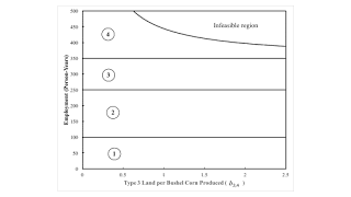
| Figure 1: A Partition of a Slice of the Parameter Space |
This post presents another example from Woods (1990). It is a modification of this example.
That previous example demonstrates that the order of fertility - the order in which lands of various types and that support different processes of production are taken into cultivation - varies with distribution. If the wage were different, the order of fertility could be different. Furthermore, the order of rentability - the order of lands from high rent to low rent - also varies with distribution. The order of fertility is not necessarily the order of rentability.
This post demonstrates another issue in the order of fertility. It depends, in this sort of open model, if one takes the wage or the rate of profits as given. This variation introduces complications in comparing the order of rentability with the order of fertility.
Some might think that those who succeed under capitalism might do so because of some physical characteristics. Those who are well off by might wonder if that is because they "are necessarily better than those who obey, and if strength of body or of mind, wisdom or virtue are always found in particular individuals, in proportion to their power or wealth: a question fit perhaps to be discussed by slaves in the hearing of their masters, but highly unbecoming to reasonable and free men in search of the truth" (Rousseau). Those who believe so are confusing social relationships between people with as relationships between things. And they just do not know price theory.
You might tell me that most mainstream economists are deluded by illusions created by competition. I would reply, "Yes, sure."
2.0 TechnologyAs previously, this is an example (Table 1) of a capitalist economy in which two commodities, iron and corn, are produced. One process is known for producing iron. In the iron industry, workers use inputs of corn to produce an output of iron. Three processes are known for producing corn. Each corn-producing process operates on a specific type of land. These processes can be thought of as examples of joint production. Their outputs are corn and the same quantity of land used as input, unchanged by the production process. Presumably, some of the labor in these processes is used to maintin the land in a given state.
| Input | Iron Industry | Corn Industry | ||
| I | II | III | IV | |
| Labor | a0,1 = 1 | a0,2 = 1/2 | a0,3 = 3 | a0,4 = 2 |
| Type 1 Land | 0 | b1,2 = 1 | 0 | 0 |
| Type 2 Land | 0 | 0 | b2,3 = 1 | 0 |
| Type 3 Land | 0 | 0 | 0 | b3,4 |
| Iron | a1,1 = 0 | a1,2 = 1/2 | a1,3 = 1/8 | a1,4 = 1/3 |
| Corn | a2,1 = 1/2 | a2,2 = 0 | a2,3 = 0 | a2,4 = 1/4 |
I complete the specification of technology with unchanged parameters for the quantities available of non-produced means of production. For this numerical example, let there be T1 = 100 acres of type 1 land, T2 = 80 acres of type 2 land, and T3 = 40 acres of type 3 land. Each process exhibits constant returns to scale, up to the limit imposed by the given quantities of the types of land.
I continue to consider stationary states with a net output consisting solely of corn. A bushel corn is the numeraire. In each possible technique, iron is produced by operating process I. Table 2 specifies which types of land are fully or partially farmed in each technique.
| Technique | Type of Land | ||
| Type 1 | Type 2 | Type 3 | |
| Alpha | Fully farmed | Fully farmed | Partially farmed |
| Beta | Partially farmed | Fully farmed | Fully farmed |
| Gamma | Fully farmed | Partially farmed | Fully farmed |
| Delta | Fully farmed | Partially farmed | Fallow |
| Epsilon | Fully farmed | Fallow | Partially farmed |
| Zeta | Partially farmed | Fully farmed | Fallow |
| Eta | Fallow | Fully farmed | Partially farmed |
| Theta | Partially farmed | Fallow | Fully farmed |
| Iota | Fallow | Partially farmed | Fully farmed |
| Kappaa | Partially farmed | Fallow | Fallow |
| Lambda | Fallow | Partially farmed | Fallow |
| Mu | Fallow | Fallow | Partially farmed |
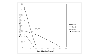
One can construct wage curves, for each of the Kappa, Lambda, and Mu techniques. In these cases, since final output is such that no type of land is fully cultivated, all rents are zero. Figure 2 depict the wage curves, with each curve labeled by the type of land that is partially farmed under the corresponding technique.
| Figure 2: Wage Curves |
These wage curves can be used to analyze rents when requirements are use are high enough such that they cannot be satisfied by only cultivating one type of land. Accordingly, suppose they can only be satisfied when farmers introduce a second type of land into cultivation, after fully farming the most fertile land. This assumption implies parameters lie within Region 3 in the analysis elaborated in Section 4.
Suppose the wage is taken as given. For a low wage, between zero and approximately 0.261 bushels per person-year, Type 2 land is the most fertile. Its wage curve lies on the outer envelope in Figure 2. So the Zeta technique will be adopted. On the other hand, consider a higher wage up to 3/10 bushels per person-year. The Delta technique, in which Type 1 land is fully cultivated and Type 2 land is partially cultivated, is cost-minimizing.
The same techniques are cost-minimizing, under these assumptions about requirements for use, if the rate of profits is taken as given. For a low rate of profits, below approximately 62 percent, the Delta technique is cost minimizing. For a higher rate of profits, up to 100 percent, farmers will adopt the Zeta technique.
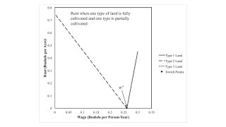
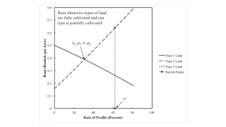
Figure 3 graphs rent against the wage. When the Zeta technique is operated, Type 2 land is fully cultivated and is the only type of land that pays a rent. The analogous conclusion holds for Type 1 land. The rate of profits increases to the left in the figure.
| Figure 3: Rent When Two Types of Land are Taken In Cultivation |
The assumption, in this example, that only one land is fully cultivated illustrates the dependence of the order of fertility on distribution. It does not allow, however, one to contrast the importance of whether the wage or the rate of profits is taken as given. Nor does it illustrate the difference between the order of fertility and the order of rentability.
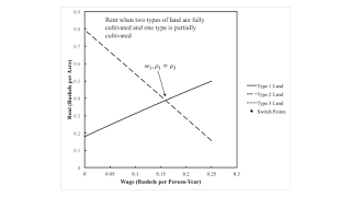
3.2 Two Types of Land Fully Cultivated, One Partially FarmedAccordingly, suppose requirements for use are such that more than two types of land must be cultivated. Which type of land is partially farmed can be determined by looking at the inner envelope of the wage curves in Figure 2. Given the wage, the order of fertility, from most fertile to least fertile, is Type 2, Type 1, and Type 3 lands. The switch point occurs at a wage exceeding the maximum wage when Type 3 lands pay no rent.
Figure 4 graphs rent versus the wage in this case. For low wages, the order of rentability, from Type 2 to Type 1 to Type 3 lands, matches the order of rentability. For high wages, the order of rentability is Type 1, Type 2, Type 3. The order of rentability no longer matches the order of fertability.
| Figure 4: Rent When Three Types of Land are Taken In Cultivation |
By constrast, suppose the rate of profits is taken as given. For low rates of profits, the order of fertility is Type 1, Type 2, Type 3. For high rates of profits, it is Type 2, Type 1, Type 3. Figure 5 graphs the rent per acre, in this case, against the rate of profits. I also indicate the location of the switch point for wage curves on this graph. The order of rentability matches the order of fertility for low and high rates of profits, but not for intermediate rates of profits.
| Figure 5: Another View of Rent When Three Types of Land are Taken In Cultivation |
I now do my usual thing of partitioning some selection of the parameter space. See Figure 1 at the top of this post. In each numbered region, the analysis of the choice of technique does not change, in some sense. Table 3 provides a brief characterization of each region, with perturbations in the given wage.
| Region | Wage | Rents | Technique | Summary |
| 1 | 0 < w < w* | ρ1 = ρ2 = ρ3 = 0 | Lambda | Type 2 partially farmed. Types 1 and 3 fallow. |
| w* < w < wmax, 1 | ρ1 = ρ2 = ρ3 = 0 | Kappa | Type 1 partially farmed. Types 2 and 3 fallow. | |
| 2 | 0 < w < w* | ρ1 = ρ2 = ρ3 = 0 | Lambda | Type 2 partially farmed. Types 1 and 3 fallow. |
| w* < w < wmax, 2 | ρ1 > 0. ρ2 = ρ3 = 0 | Delta | Type 1 fully farmed. Type 2 partially farmed. Type 3 fallow. | |
| 3 | 0 < w < w* | ρ2 > 0. ρ1 = ρ3 = 0 | Zeta | Type 2 fully farmed. Type 1 partially farmed. Type 3 fallow. |
| w* < w < wmax, 2 | ρ1 > 0. ρ2 = ρ3 = 0 | Delta | Type 1 fully farmed. Type 2 partially farmed. Type 3 fallow. | |
| 4 | 0 < w < w1 | ρ2 > ρ1 > 0. ρ3 = 0 | Alpha | Order of rentability matches order of fertility, given wage. |
| w1 < w < wmax, 3 | ρ1 > ρ2 > 0. ρ3 = 0 | Alpha | Order of rentability differs from order of fertility, given wage. |
Section 3 emphasizes that how the choice of technique is analyzed depends on whether or not the wage or the rate of profits is taken as given. Table 4 describes the regions in Figure 1, assuming the rate of profits is given. The interesting aspect of these tables comes from contrasting the description of Region 4 in Tables 3 and 4.
| Region | Rate of Profits | Rents | Technique | Summary |
| 1 | 0 < r < r* | ρ1 = ρ2 = ρ3 = 0 | Kappa | Type 1 partially farmed. Types 2 and 3 fallow. |
| r* < r < rmax, 2 | ρ1 = ρ2 = ρ3 = 0 | Lambda | Type 2 partially farmed. Types 1 and 3 fallow. | |
| 2 | 0 < r < r* | ρ1 > 0. ρ2 = ρ3 = 0 | Delta | Type 1 fully farmed. Type 2 partially farmed. Type 3 fallow. |
| r* < r < rmax, 2 | ρ1 = ρ2 = ρ3 = 0 | Lambda | Type 2 partially farmed. Types 1 and 3 fallow. | |
| 3 | 0 < r < r* | ρ1 > 0. ρ2 = ρ3 = 0 | Delta | Type 1 fully farmed. Type 2 partially farmed. Type 3 fallow. |
| r* < r < rmax, 1 | ρ2 > 0. ρ1 = ρ3 = 0 | Zeta | Type 2 fully farmed. Type 1 partially farmed. Type 3 fallow. | |
| 4 | 0 < r < r1 | ρ1 > ρ2 > 0. ρ3 = 0 | Alpha | Order of rentability matches order of fertility, given rate of profits. |
| r1 < r < r* | ρ2 > ρ1 > 0. ρ3 = 0 | Alpha | Order of rentability differs from order of fertility, given rate of profits. | |
| r* < r < rmax, 3 | ρ2 > ρ1 > 0. ρ3 = 0 | Alpha | Order of rentability matches order of fertility, given rate of profits. |
This post is not about what is wrong with aggregating capital. Nor is it about aggregate production functions. It is an exploration of an open model, and this model is therefore not a marginalist general equilibrium model. It synthesizes some ideas in Sraffa (1925) and Sraffa (1960). I think especially of Sraffa's comments on Wicksteed's distinction between descriptive and functional curves, between spurious and genuine margins.
References- Piero Sraffa. 1925. Relazioni fra costo e quantita prodotta. Annali di Economia 2. Trans. by A. Roncaglia and J. Eatwell.
- Piero Sraffa. 1960 The Production of Commodities by Means of Commodities Cambridge University Press.
- J. E. Woods. 1990. The Production of Commodities: An Introduction to Sraffa. Atlantic Highlands: Humanities Press.
 Heterodox

