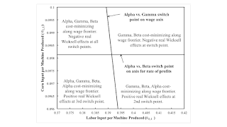
Figure 1: A Part of the Parameter Space1.0 Introduction This post presents a perturbation of an example from Salvatore Baldone. It follows the style of some posts that almost add up to a draft research paper. A widespread view among Austrian-school and mainstream economists is mistaken. Given competitive markets, if the supply of capital were increased, in some sense, the rate of profits would supposedly be driven down. At the level of abstraction here, no distinction exists between the interest rate and the rate of profits. A lower rate of profits would incentivize capitalists to adopt more capital-intensive techniques and thereby increase the output produced per worker. A more capital-intensive technique is supposed to be associated with an increased period of production. Some such
Topics:
Robert Vienneau considers the following as important: Austrian School Of Economics, Example in Mathematical Economics, Joint Production, Sraffa Effects
This could be interesting, too:
Robert Vienneau writes Austrian Capital Theory And Triple-Switching In The Corn-Tractor Model
Robert Vienneau writes Double Fluke Cases For Triple-Switching In The Corn-Tractor Model
Robert Vienneau writes The Emergence of Triple Switching and the Rarity of Reswitching Explained
Robert Vienneau writes Recap For A Triple -Switching Example
| Figure 1: A Part of the Parameter Space |
This post presents a perturbation of an example from Salvatore Baldone. It follows the style of some posts that almost add up to a draft research paper.
A widespread view among Austrian-school and mainstream economists is mistaken. Given competitive markets, if the supply of capital were increased, in some sense, the rate of profits would supposedly be driven down. At the level of abstraction here, no distinction exists between the interest rate and the rate of profits. A lower rate of profits would incentivize capitalists to adopt more capital-intensive techniques and thereby increase the output produced per worker. A more capital-intensive technique is supposed to be associated with an increased period of production. Some such regularity seems to me to be necessary to make sense out of Austrian Business Cycle Theory.
This post presents a perturbation of an example in which net output conisists of a single commodity. Capital inputs are heterogeneous. One input consists of a machine. Sometimes truncating the economic life of the machine results in a more capital-intensive technique of production. This post emphasizes the disconnection between capital-intensity and physical properties of how long machinery is operated by capitalists maximizing their profits.
2.0 TechnologyTable 1 presents coefficients of production in a perturbation of an example from Baldone (1974). With the first process, workers, under the direction of mangers of firms, manufacture new machines. The remaining three processes are used to produce corn. The second process requires an input of a new machine, as well as seed corn. A one-year old machine is jointly produced with the output of corn. The third process jointly produces an output of a two-year old machine with corn. The fourth process exhausts the physical life of the machine. Only corn is produced as a output in this process.
| Input | Industry | Agriculture | ||
| I | II | III | IV | |
| Labor | a0,1 | 39/200 | 117/200 | 39/100 |
| Corn | a1,1 | 39/100 | 141/250 | 117/200 |
| New Machines | 0 | 1 | 0 | 0 |
| 1-Year Old Machines | 0 | 0 | 1 | 0 |
| 2-Year Old Machines | 0 | 0 | 0 | 1 |
| Output | ||||
| Corn | 0 | 1 | 1 | 1 |
| New Machines | 1 | 0 | 0 | 0 |
| 1-Year Old Machines | 0 | 1 | 0 | 0 |
| 2-Year Old Machines | 0 | 0 | 1 | 0 |
Corn is both a consumption good and a capital good, insofar as it is an input into all four processes. Technology is not yet fully specified in this example, with numerical values undefined for two coefficients of production. I assume free disposal of old machines. The choice of technique here is equivalent to the choice of the economic life of the machine. Table 2 lists the processes operated for the available techniques, each of which can produce a net output of one bushel corn. Under Alpha, the machine is junked after operating one year. Under Beta, it is junked after two years. Under Gamma, it is operated for its full physical life.
| Technique | Processes |
| Alpha | I, II |
| Beta | I, II, III |
| Gamma | I, II, III, IV |
The economic life of the machine is chosen on the basis of cost-minimization. Accordingly, I consider prices of production for each technique. A bushel corn is numeraire. I assume that wages are paid out of the surplus product at the end of the year. Each operated process yields the same rate of profits.
These assumptions are enough to derive, for each technique, wages and prices as functions of the rate of profits. Three equivalent methods can be used to find the cost-minimizing technique at any given rate of profits:
- Construct the wage frontier as the outer envelope of the wage curves for the technique. This is a pure fixed capital example.
- Look for negative prices for old machines. Beta cannot be cost minimizing if a one-year old machine has a negative price at prices of production for the Beta technique. Gamma cannot be cost-minimizing if a two-year old machine has a negative price at Gamma prices.
- Determine if extra profits can be made by adopting a process not operated in calculating prices of production. Does operating the machine for two years yield extra profits at Alpha prices? For three years at Beta prices?
For the pure fixed capital model, these three methods of analyzing the choice of technique are equivalent. In the general case of joint production, the outer envelope of the wage curves does not always correspond to the cost-minimizing technique.
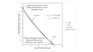
4.0 Two Fluke Points and the Perturbation of Coefficients of ProductionFigure 2 illustrates the analyis of the choice of technique for the specified values of the direct labor input and corn input, per machine produced in the industrial process. A switch point between Beta and Gamma exists at approximately 61 percent. Around this switch point, a lower rate of profits is associated with an extension of the economic lifetime of the machine and an increased output per worker. Score one for Böhm Bawerk. These parameters have been carefully chosen to yield two fluke switch points with Alpha, one at the maximum wage and one at the maximum rate of profits. Aside from these flukes, this example seems straightforward.
| Figure 2: An Example Of Two Fluke Switch Points |
I now consider local perturbations of these two coefficients of production. Figure 1, at the top of this post, depicts the part of the parameter space under consideration. The machine varies in efficiency as it is used in agriculture, and these perturbations leave unchanged the needed inputs of labor and corn to operate with the machine at each age. The parameters partition the parameter space around the fluke case in Figure 2. The wage frontier does not differ qualitatively in each of these four regions, but it does differ among regions.
The wage frontier to the northeast looks like the frontier in Figure 2, but the switch points on the axis for the wage or the rate of profits no longer appear. As noted, the single switch point between Beta and Gamma conforms to outdated Austrian and marginalist intuition.
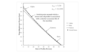
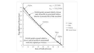
5.0 Non-Monotonic Economic Lifetime of a Machine to the NorthwestThe region to the northwest, as illustrated in Figure 3, is more interesting. This is not a reswitching example. Nor is it an example of capital-reversing in this region of the parameter space. Prices can be used to evaluate the payments made for advances for capital inputs for each technique. Around the two switch points, a lower rate of profits is associated with a larger value of capital per unit output for the newly cost-minimizing technique. More capital per worker is used, and output per worker is increased. With a lower rate of profits, the machine is operated two years, three years, and then one year. At the first switch point, a shorter economic life of a machine is associated with greater capital-intensity. This result seems to pose some difficulty for traditional formulations of Austrian capital theory.
| Figure 3: An Example Of Non-Monotonic Variations in the Economic Life of a Machine |
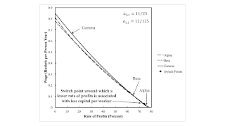
Figure 4 illustrates the region in the parameter space to the southeast. This is an example of capital-reversing but not of the reswitching of techniques. The wage curves for the Alpha and Beta techniques intersect twice, with the first intersection within the wage frontier. Around the second switch point, a lower rate of profits associated with a smaller value of capital per unit output. Less capital per worker is used, and output per worker is lower at a lower rate of profits. Long run marginalist theory is falsified. With a lower rate of profits, the machine is operated one year, two years, and then three years. At the second switch point, a longer economic of a machine is associated with a decrease in capital-intensity. Austrian capital theory is not validated here, either.
| Figure 4: An Example Of Capital-Reversing |
In the southwest, both these difficulties for Austrian capital theory arise, as illustrated in Figure 5. This is now a reswitching example. At a low or high rate of profits, the machine is operated for one year. The interval of the rate of profits between these two intervals in which Alpha is cost-minimized are partitioned by another switch point. Gamma is cost-minimizing in one partition, and Beta is cost-minimizing in the other. At the first switch point, a shorter economic life of the machine is associated with a lower rate of profits and the adoption of a more capital-intensive technique. At the third switch point, a longer economic life of a machine is associated with a smaller rate of profits and a decrease in capital-intensity.
| Figure 5: A Reswitching Example |
Harwick (2022) has noted that some followers of the Austrian school have recently tried to consider Austrian capital theory separately from business-cycle theory. Lewin and Cachanosky (2019) consider a financial measure of capital-intensity, namely the average duration of an investment project. Around any switch point, an increased Duration is (tautologically?) associated with a lower interest rate. As noted by Fratini (2019), an increased capital intensity, in this sense, is associated with reduced net output per worker around a so-called 'perverse' switch point. Noting that a technique exhibiting joint production cannot always be reduced to an infinite series of dated labor inputs, I do not know how to calculate Duration for the above example. (Those wanting to address this implicit challenge might want to start with this example to warmup.) But even so, an increased Duration can be associated with the reduction in the economic life of a machine.
Anyways, a reduction in the economic life of a machine is consistent with an increase in capital-intensity. Capital-intensity is assessed above by evaluating the price of inputs, either for a given net output or per worker. This association between a shorter economic life and greater capital-intensity can arise around a switch point in which a smaller rate of profits incentives the adoption of a more capital-intensive technique, with a consequent greater net output per worker. It can also arise around a ‘perverse’ switch point in which a less capital-intensive technique is adopted at a lower rate of profits. Neither type of switch point is a fluke case, as can be seen by contrasting such switch points with genuine fluke cases.
Reference- Salvatore Baldone. 1974. Il capitale fisso nello schema teorico di Piero Sraffa. Studi Economici XXIV(1): 45-106. Translated in Pasinetti (1980).
- Saverio M. Fratini. 2019. A note on re-switching, the average period of production and the Austrian business-cycle theory. Review of Austrian Economics 32: 363-374.
- Cameron Harwick. 2022. Unmixing the metaphors of Austrian capital theory. Review of Austrian Economics 35: 163-176.
- Peter Lewin and Nicholas Cachanosky. 2019. Austrian Capital Theory: A Modern Survey of the Essentials. Cambridge: Cambridge University Press.
 Heterodox

