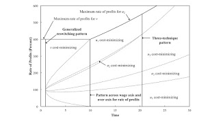
Figure 1: Switch Points Varying with Time1.0 Introduction This post presents a perturbation of a fluke switch point. At this switch point, the wage curves for four techniques are tangent. In the jargon I have been inventing, this is another four-technique, local pattern. In other words, a perturbation of appropriately selected parameters - for example, coefficients of production - changes the sequence of wage curves and switch points on the wage frontier. The perturbation can be viewed as the result of technical progress. When I worked the example, I was surprised to find some other fluke cases. The numeric example is an instance of the Samuelson-Garegnani model. Of interest to me, is a generalization to a continuum of techniques with wage curves tangent at the switch point. A
Topics:
Robert Vienneau considers the following as important: Example in Mathematical Economics, Sraffa Effects
This could be interesting, too:
Robert Vienneau writes Austrian Capital Theory And Triple-Switching In The Corn-Tractor Model
Robert Vienneau writes Double Fluke Cases For Triple-Switching In The Corn-Tractor Model
Robert Vienneau writes The Emergence of Triple Switching and the Rarity of Reswitching Explained
Robert Vienneau writes Recap For A Triple -Switching Example
|
| Figure 1: Switch Points Varying with Time |
This post presents a perturbation of a fluke switch point. At this switch point, the wage curves for four techniques are tangent. In the jargon I have been inventing, this is another four-technique, local pattern. In other words, a perturbation of appropriately selected parameters - for example, coefficients of production - changes the sequence of wage curves and switch points on the wage frontier. The perturbation can be viewed as the result of technical progress. When I worked the example, I was surprised to find some other fluke cases.
The numeric example is an instance of the Samuelson-Garegnani model. Of interest to me, is a generalization to a continuum of techniques with wage curves tangent at the switch point. A perturbation leads to an example with no switch points, but the cost-minimizing technique varies continuously along the wage frontier, and techniques recur. So this generalization will have the structure of an example in Garegnani (1970). Kurz and Salvador (2003) later simplified this famous example. In some sense, I am offering a further simplification. But, perhaps, my example is more complicated along other dimensions, insofar as my pattern analysis is original.
2.0 TechnologyIn this economy, a single consumption good - called corn - is produced from inputs of labor and a specified grade of iron. The grade of iron is indexed by v, u1, u2, and u3. Each grade of iron is itself produced from inputs of labor and that grade of iron. Table 1 shows the processes available, at each point in time, for producing iron. Similarly, Table 2 defines the processes available for producing corn. This is a circulating capital model. The iron inputs are totally used up in a single production period.
| Input | Process | |||
| v | u1 | u2 | u3 | |
| Labor | (2/5) | (5/18)e-(t - 1)σ1 | (49/360)e-(t - 1)σ2 | (2/45)e-(t - 1)σ3 |
| v Iron | (1/5) | 0 | 0 | 0 |
| u1 Iron | 0 | (1/4)e-(t - 1)σ1 | 0 | 0 |
| u2 Iron | 0 | 0 | (13/40)e-(t - 1)σ2 | 0 |
| u3 Iron | 0 | 0 | 0 | (2/5)e-(t - 1)σ3 |
| Input | Process | |||
| v | u1 | u2 | u3 | |
| Labor | 2 | (20/9) | (23/9) | (26/9) |
| v Iron | 1 | 0 | 0 | 0 |
| u1 Iron | 0 | 1 | 0 | 0 |
| u2 Iron | 0 | 0 | 1 | 0 |
| u3 Iron | 0 | 0 | 0 | 1 |
Four techniques for producing a net output of corn exist. Each technique consists of a process for producing iron of a specific grade and a process for producing corn with that grade of iron. For my notes when extending this example to a continuum of techniques, I want to note the following restriction and relationships among coefficients of production:
(1/5) ≤ a1,1(u, 1) < (1/2)
a0,1(u, 1) = (10/9)[1 - 2 a1,1(u, 1)]2
a0,2(u, 1) = (10/9)[1 + 4 a1,1(u, 1)]3.0 Prices
Suppose the technique defined by the u grade of iron is in use. Consider the associated prices of production, for the period of production ending at time t. Let r be the rate of profits, wu(r, t) be the wage, and pu(r, t) the price of u-grade iron. Prices are production satisfy the following system of two equations:
pu(r, t) a1,1(u, t) R + a0,1(u, t) wu(r, t) = pu(r, t)
pu(r, t) R + a0,2(u, t) wu(r, t) = 1
where:
R = 1 + r
A bushel corn is the numeraire.
One can solve this system for the wage and the price of corn, each as a function of the rate of profits and time. The wage, as a function of the rate of profits, is called the wage curve for the technique. A different wage curve is defined for the technique defined by each grade of iron. The wage curve for the v-grade of iron does not shift with time.
4.0 Choice of TechniqueThe wage curves, for each of the techniques defined by a grade of iron, can be plotted on the same graph. This graph depicts wage curves and the wave frontier at a given point in time. The wage frontier is the outer envelope of the wage curves. The technique(s) that contribute their wage curve(s) to the frontier are cost minimizing for the corresponding rate of profits or wage.
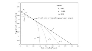
4.1 The Wage Frontier at t = 1Figure 2 shows the wage frontier at t = 1. The technique defined by v-grade iron is cost-minimizing for all feasible rates of profits. All four techniques are cost-minimizing at the single switch point. All four wage curves are tangent at the switch point. This is a fluke.
|
| Figure 2: Wage Curves Tangent at Switch Points |
In Figure 2, I have indicated the rate of technical progress for the three techniques defined by u1, u2, and u3. But, with the way I have defined technical progress, these rates do not matter for prices of production at time t = 1. Furthermore, for any time less than unity, the wage frontier is the same. The wage curve for v-grade iron does not shift, and the technique defined by v-grade iron is uniquely cost-minimizing for all feasible rates of profits. The story is different for as time goes on after t = 1.
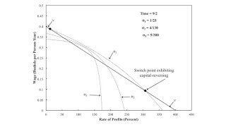
4.2 The Shift in Wage Frontier when Technical Change is Faster for Smaller a1,1(u, 1)First, consider the case when σ is smaller for a larger index u for the grade of iron. Figure 3 graphs such a case, for a time larger than t = 1. This is an example of reswitching, between the techniques defined by v-grade and u1-grade iron. The wage curves for the techniques defined for u2-grade and u3-grade iron appear on the frontier only at t = 1 and only at the switch point. Otherwise, this is a perturbation analysis, for these rates of technical progress, that yields a traditional reswitching example.
|
| Figure 3: A Reswitching Example |
I created this example more with this case in mind. In obvious notation, define the rates of technical progress by:
σu = (1/10) a1,1(u, 1)
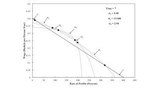
Figure 4 graphs the wage frontier shortly after t = 1. The wage curves for the techniques defined by v-grade, u1, and u2 each appear in two separate regions on the wage frontier. The single switch point has become six switch points. Perturbation of the coefficients of production for the fluke switch point has yielded an example of the recurrence of techniques.
|
| Figure 4: Recurrence of Techniques |
Around the three switch points at the larger rates of profits, a higher wage is associated with the adoption of a cost-minimizing technique where more labor is employed per unit of the consumption good produced. When will mainstream economists stop telling lies to students about price theory and the logic of minimum wages?
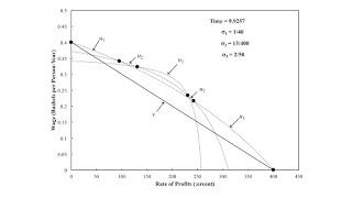
Figure 5 graphs the wage frontier at the following time:
t = 1 - 40 ln(4/5)
This is an example that is simultaneously a pattern across the wage axis and over the axis for the rate of profits. The technique defined by v-grade iron, and the associated switch points, is disappearing from the wage frontier. I did some work to previously create such a global pattern. I do not know what specific, presumably special case conditions, I have imposed to make this pattern come about. These numeric examples keep
|
| Figure 5: Switch Points on Both Axes |
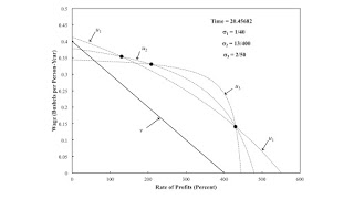
Figure 6 graphs the wage frontier at an even later point in time. Three switch points appear on the frontier. Three wage curves intersect at the switch point at the larger rate of profits. This is what I call a three-technique pattern. The wage curve for the u2-grade iron is disappearing from the wage frontier.
|
| Figure 6: A Three-Technique Pattern |
The diagram at the top of this post summarizes my analysis for this case. The rates of profits for switch points are plotted against time. The maximum rate of profits is also shown.
5.0 ConclusionI have exhibited a numerical example in which four-wage curves are tangent at a single switch point. Technical progress alters certain parameters - that is, coefficients of production - for three of the four techniques. For any time less than the time at which the fluke switch point occurs, no switch point exists. Given a certain simple specification of the rates of technical progress, the switch point breaks up into six switch points for a small increase in time. Three of the four technique recur on the wage frontier. In my jargon, the fluke case is a four-technique pattern. It generalizes the reswitching pattern I have previously defined. I claim that I can create a n-technique generalized reswitching pattern, for any finite n greater than unity. I can also create generalized reswitching pattern with a continuum of wage curves tangent at the single switch point.
My next steps, if I go on, might be to explicitly write up the generalization to a continuum of techniques. I should also find a closed-form for the time at which the above three-technique pattern occurs. (I found it through a bisection algorithm.)
References- P. Garegnani (1970). Heterogeneous Capital, the Production Function and the Theory of Distribution. Review of Economic Studies, V. 37, no. 3: pp. 407-436.
- Heinz D. Kurz and Neri Salvadori (2003). Reswitching - Simplifying a Famous Example. In Kurz and Salvadori (eds.) Classical Economics and Modern Theory: Studies in Long-Period Analysis Routledge.
 Heterodox
