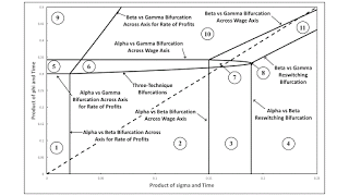
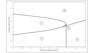
Figure 1: A Bifurcation Diagram This post expands on this previous post. The technology is the same, but the rates of decrease of the coefficients of production in the Beta and Gamma corn-producing processes are not fixed. Instead, I consider the full range of parameter values. (I find the graphs produced by bifurcation analysis interesting for this case, but I think a two-commodity example can be found with more pleasing diagrams.) Anyways, Figure 1 shows a bifurcation diagram for the parameter space in this example. The region numbered 8 is not visible on the graph. Accordingly, Figure 2 below shows a much expanded picture of the parameter space around that region. The specific parameter values in the previous post lead to a temporal path along the dashed ray extending from the
Topics:
Robert Vienneau considers the following as important: Example in Mathematical Economics, Sraffa Effects, Towards Complex Dynamics
This could be interesting, too:
Robert Vienneau writes Austrian Capital Theory And Triple-Switching In The Corn-Tractor Model
Robert Vienneau writes Double Fluke Cases For Triple-Switching In The Corn-Tractor Model
Robert Vienneau writes The Emergence of Triple Switching and the Rarity of Reswitching Explained
Robert Vienneau writes Recap For A Triple -Switching Example

|
| Figure 1: A Bifurcation Diagram |
This post expands on this previous post. The technology is the same, but the rates of decrease of the coefficients of production in the Beta and Gamma corn-producing processes are not fixed. Instead, I consider the full range of parameter values. (I find the graphs produced by bifurcation analysis interesting for this case, but I think a two-commodity example can be found with more pleasing diagrams.)
Anyways, Figure 1 shows a bifurcation diagram for the parameter space in this example. The region numbered 8 is not visible on the graph. Accordingly, Figure 2 below shows a much expanded picture of the parameter space around that region. The specific parameter values in the previous post lead to a temporal path along the dashed ray extending from the origin in Figure 1. (The numbering of regions in this post and the previous post do not correspond.) Although it is not obvious, the locus of points bifucating regions 9 and 10 eventually, somewhere to the right of the region shown in Figure 1 eventually decreases in slope and intercepts the dashed ray.

|
| Figure 2: Blowup of a Part of the Bifurcation Diagram |
As usual, each numbered region corresponds to a definite sequence of cost-minimizing techniques contributing wage curves along the wage frontier. Table 1 lists this sequence for each region. Some notes on switch points are provided. A switch point is called "normal" merely if it conforms to outdated neoclassical intuition. In other words, such a switch point exhibits negative real Wicksell effects. In the example, regions also exist where switch points exhibit positive real Wicksell effects.
| Region | Cost-Minimizing Techniques | Notes |
| 1 | Alpha | One technique cost-minimizing. |
| 2 | Alpha, Beta | "Normal" switch point. |
| 3 | Beta, Alpha, Beta | Reswitching. Switch pt. at highest r is "perverse". |
| 4 | Beta | One technique cost-minimizing. |
| 5 | Alpha, Gamma | "Normal" switch point. |
| 6 | Alpha, Gamma, Beta | "Normal" switch points. |
| 7 | Beta, Alpha, Gamma, Beta | Recurrence of techniques. Switch pt. at highest r is "perverse". |
| 8 | Beta, Alpha, Beta, Gamma, Beta | Two reswitchings, two "perverse" switch pts. |
| 9 | Gamma | One technique cost-minimizing. |
| 10 | Gamma, Beta | "Normal" switch point. |
| 11 | Beta, Gamma, Beta | Reswitching. Switch pt. at highest r is "perverse". |
One can compare and contrast the above bifurcation diagram with the one in this post. The latter bifurcation diagram is for a specific instance of the Samuelson-Garegnani model, in which the basic commodity varies among techniques. (I have a more recent write-up of that bifurcation analysis linked to here.)
 Heterodox
