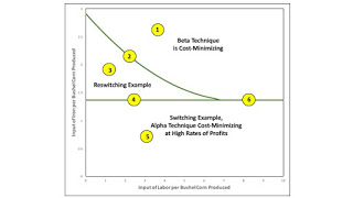
Figure 1: Bifurcation Diagram This post is a continuation of the analysis in this reswitching example. That post presents an example of reswitching in a model of the production of commodities by means of commodities. The example is one of an economy in which two commodities, iron and corn, are produced. Managers of firms know of two processes for producing iron and one process for producing corn. The definition of technology results in a choice between two techniques of production. The two-commodity model analyzed here is specified by nine parameters. Theoretically, a bifurcation diagram should be drawn in nine dimensions. But, being limited by the dimensions of the screen, I select two parameters. I take the inputs per unit output in the two processes for producing iron as given
Topics:
Robert Vienneau considers the following as important: Example in Mathematical Economics, Sraffa Effects, Towards Complex Dynamics
This could be interesting, too:
Robert Vienneau writes Austrian Capital Theory And Triple-Switching In The Corn-Tractor Model
Robert Vienneau writes Double Fluke Cases For Triple-Switching In The Corn-Tractor Model
Robert Vienneau writes The Emergence of Triple Switching and the Rarity of Reswitching Explained
Robert Vienneau writes Recap For A Triple -Switching Example

|
| Figure 1: Bifurcation Diagram |
This post is a continuation of the analysis in this reswitching example. That post presents an example of reswitching in a model of the production of commodities by means of commodities. The example is one of an economy in which two commodities, iron and corn, are produced. Managers of firms know of two processes for producing iron and one process for producing corn. The definition of technology results in a choice between two techniques of production.
The two-commodity model analyzed here is specified by nine parameters. Theoretically, a bifurcation diagram should be drawn in nine dimensions. But, being limited by the dimensions of the screen, I select two parameters. I take the inputs per unit output in the two processes for producing iron as given constants. I also take as given the amount of (seed) corn needed to produce a unit output of corn, in the one process known for producing corn. So the dimensions of my bifurcation diagram are the amount of labor required to produce a bushel corn and the amount of iron input required to produce a bushel corn. Both of these parameters must be non-negative.
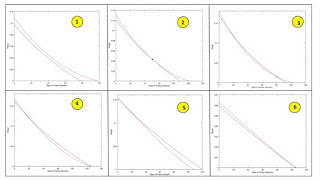
I am interested in wage curves and, in particular, how many intersections they have. Figure 1, above, partitions the parameter space based on this rationale. I had to think some time about what this diagram implies for wage curves. In generating the points to interpolate, my Matlab/Octave code generated many graphs analogous to those in the linked post. I also generated Figure 2, which illustrates configurations of wage curves and switch points, for the number regions and loci in Figure 1. So I had some visualization help, from my code, in thinking about these implications. Anyways, I hope you can see that, from perturbations of one example, one can generate an infinite number of reswitching examples.

|
| Figure 2: Some Wage Curves |
One can think of prices of production as (not necessarily stable) fixed points of short period dynamic processes. Economists have developed a number of dynamic processes with such fixed points. But I leave my analysis open to a choice of whatever dynamic process you like. In some sense, I am applying bifurcation analysis to the solution(s) of a system of algebraic equations. The closest analogue I know of in the literature is Rosser (1983), which is, more or less, a chapter in his well-known book.
Update (22 Jun 2017): Added Figure 2, associated changes to Figure 1, and text.
References- J. Barkley Rosser (1983). Reswitching as a Cusp Catastrophe. Journal of Economic Theory V. 31: pp. 182-193.
 Heterodox
