Figure 1: A Bifurcation Diagram I have previously illustrated a case in which real Wicksell effects are zero. I wrote this post to present an argument that that example is not a matter of round-off error confusing me. Consider the technology illustrated in Table 1. The managers of firms know of three processes of production. These processes exhibit Constant Returns to Scale. The column for the iron industry specifies the inputs needed to produce a ton of iron. Two processes are known for producing corn, and their coefficients of production are specified in the last two columns in the table. Each process is assumed to require a year to complete and uses up all of its commodity inputs. Table 1: The Technology InputIndustryIronCornAlphaBeta
Topics:
Robert Vienneau considers the following as important: Example in Mathematical Economics, Sraffa Effects
This could be interesting, too:
Robert Vienneau writes Austrian Capital Theory And Triple-Switching In The Corn-Tractor Model
Robert Vienneau writes Double Fluke Cases For Triple-Switching In The Corn-Tractor Model
Robert Vienneau writes The Emergence of Triple Switching and the Rarity of Reswitching Explained
Robert Vienneau writes Recap For A Triple -Switching Example
|
| Figure 1: A Bifurcation Diagram |
I have previously illustrated a case in which real Wicksell effects are zero. I wrote this post to present an argument that that example is not a matter of round-off error confusing me.
Consider the technology illustrated in Table 1. The managers of firms know of three processes of production. These processes exhibit Constant Returns to Scale. The column for the iron industry specifies the inputs needed to produce a ton of iron. Two processes are known for producing corn, and their coefficients of production are specified in the last two columns in the table. Each process is assumed to require a year to complete and uses up all of its commodity inputs.
| Input | Industry | ||
| Iron | Corn | ||
| Alpha | Beta | ||
| Labor | 1 | a0,2α | 305/494 |
| Iron | 9/20 | 1/40 | 3/1976 |
| Corn | a2,1 | 1/10 | 229/494 |
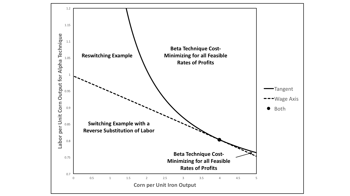
Figure 1 shows two loci in the parameter space defined by the two coefficients of production a0,2α and a2,1. The solid line represents coefficients of production for which the wage curves for the two techniques are tangent at a point of intersection. The dashed line represents parameters for which a switch point exists on the wage axis. The point at which these two loci are tangent specifies the parameters for this example. Figure 2 repeats the graph of the wage curves for that example.

|
| Figure 2: A Fluke Switch Point |
Suppose coefficients are as in the example in the main text, but a0,2α is somewhat greater. Then the wage curve for the Alpha technique lies below the wage curve for Beta for all non-negative rates of profits not exceeding the maximum rate of profits. For all feasible rate of profits, Beta is cost-minimizing. On the other hand, if a0,2α is somewhat less than in the example, the wage curve for Alpha is somewhat higher than in Figure 2. The wage curve for Alpha will intersect the wage curve for Beta at two points, one with a negative rate of profits exceeding one hundred percent and one for a switch point with a positive rate of profit. As indicated in Figure 1, this combination of parameters is an example of the reserve substitution of labor
In the region graphed in Figure 1, if the coefficient of production a0,2α falls below the loci at which the two wage curves are tangent, the wage curves will have two intersections. Suppose a2,1 is greater than in the example in the main text. In the corresponding region between the two loci in Figure 1, the rate of profits at both intersections of the wage curves are negative. In this region of the parameter space, Beta remains cost-minimizing for all feasible non-negative rates of profits. If a2,1 is less than in the example, the rate of profits for both intersections are positive in the region between the two loci. The example is one of reswitching. In effect, which intersection of the wage curves is a switch point on the wage axis changes along the locus for the switch point on the wage axis.
Consider the rate of profits at which the wage curves have a repeated intersection, that is, are tangent, for the corresponding locus in Figure 1. Toward the left of the figure, this rate of profits is positive, while it is negative toward the right. By continuity, this rate of profits is zero for a single point in the graphed part of the parameter space. The two loci must be tangent for this set of parameters. The appearance of a switch point with a real Wicksell effect of zero in this post is not a result of round-off error or finite precision arithmetic. Such a point exists for exactly specified coefficients of production.