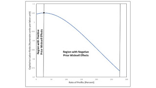
Figure 1: Price Wicksell Effects in Example1.0 Introduction This post presents another example from my on-going simulation experiments. I am still focusing on simple models without the choice of technique. The example illustrates an economy in which price Wicksell effects are positive, for some ranges of the rate of profits, and negative for another range. 2.0 Technology I used my implementation of the Monte-Carlo method to generate 20,000 viable, random economies in which three commodities are produced. For the 316 of these 20,000 economies in which price Wicksell effects are both negative and positive, the maximum vertical distance between the wage curve and an affine function is approximately 15% of the maximum wage. The example presented in this post is for that maximum. The
Topics:
Robert Vienneau considers the following as important: Example in Mathematical Economics, Sraffa Effects
This could be interesting, too:
Robert Vienneau writes Austrian Capital Theory And Triple-Switching In The Corn-Tractor Model
Robert Vienneau writes Double Fluke Cases For Triple-Switching In The Corn-Tractor Model
Robert Vienneau writes The Emergence of Triple Switching and the Rarity of Reswitching Explained
Robert Vienneau writes Recap For A Triple -Switching Example

|
| Figure 1: Price Wicksell Effects in Example |
This post presents another example from my on-going simulation experiments. I am still focusing on simple models without the choice of technique. The example illustrates an economy in which price Wicksell effects are positive, for some ranges of the rate of profits, and negative for another range.
2.0 TechnologyI used my implementation of the Monte-Carlo method to generate 20,000 viable, random economies in which three commodities are produced. For the 316 of these 20,000 economies in which price Wicksell effects are both negative and positive, the maximum vertical distance between the wage curve and an affine function is approximately 15% of the maximum wage. The example presented in this post is for that maximum.
The economy is specified by a process to produce each commodity and a commodity basket specifying the net output of the economy. Since the level of output is specified for each industry, no assumption is needed on returns to scale, I gather. But no harm will come from assuming Constant Returns to Scale (CRS). All capital is circulating capital; no fixed capital exists. All capital goods used as inputs in production are totally used up in producing the gross outputs. The capital goods must be replaced out of the harvest each year to allow production to continue on the same scale. The remaining commodities in the annual harvest constitute the given net national income. I assume the economy is in a stationary state. Workers advance their labor. They are paid wages out of the harvest at the end of the year. Net national income is taken as the numeraire.
Table 1 summarizes the technique in use in this example. The 3x3 matrix formed by the first three rows and columns is the Leontief input-output matrix. Each entry shows the physical quantity of the row commodity needed to produce one unit output of the column commodity. For example, 0.5955541 pigs are used each year to produce one bushel of corn. The last row shows labor coefficients, that is, the physical units of labor needed to produced one unit output of each commodity. The last column is net national income, in physical units of each commodity.
| Input | Corn Industry | Pigs Industry | Ale Industry | Net Output |
| Corn | 0.0905726 | 0.0021651 | 0.0022885 | 0.274545 |
| Pigs | 0.5955541 | 0.2231379 | 0.0054569 | 0.097880 |
| Ale | 0.1202180 | 0.6362278 | 0.0232452 | 0.804348 |
| Labor | 0.26273 | 0.18555 | 0.31306 |
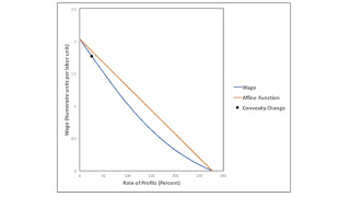
I now consider stationary prices such that the same rate of profits is made in each industry. The system of equations allow one to solve for the wage, as a function of a given rate of profits. The blue curve in Figure 2 is this wage curve. The maximum rate of profits, achieved when the wage is zero, is approximately 276.5%. The maximum wage, for a rate of profits of zero, is approximately 2.0278 numerate units per labor unit. As a contrast to the wage curve, I also draw a straight line, in Figure 2, connecting these maxima.

|
| Figure 2: Wage Curve in Example |
I do not think it is easy to see in the figure, but the wage curve is not of one convexity. The convexity changes at a rate of profits of approximately 25.35%, and I plot the point at which the convexity changes.
4.0 The Numeraire Value of Capital GoodsSince I have specified the net national product, the gross national product can be found from the Leontief input-output matrix. The gross national product is the sum of the capital goods, in a stationary state, and the net national product. The employed labor force can be found from labor coefficients and gross national product.
Given the rate of profits, one can find prices, as well as the wage. And one can use these prices to calculate the numeraire value of capital goods. Figure 1, at the top of this post, graphs the ratio of the value of capital goods to the employed labor force, as a function of the rate of profits.
A traditional, incorrect neoclassical idea is that a lower rate of profits incentivizes firms to increase the ratio of capital to labor. And a higher wage also incentivizes firms to increase the ratio of capital to labor. The region, for a low rate of profits, in which price Wicksell effects are positive already poses a problem for this vague neoclassical idea.
5.0 ConclusionThis example makes me feel better about my simulation approach. From some previous results, I was worried that I would have to rethink how I generate random coefficients. But, maybe if I generate enough economies, even with all coefficients, etc. confined to the unit interval, I will be able to find examples that approach visually interesting counter-examples to neoclassical economics.
 Heterodox
