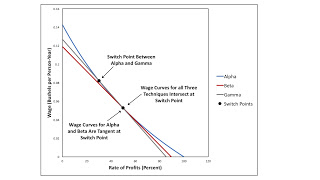
Figure 1: Wage Curves1.0 Introduction This post presents an example of the analysis of the choice of technique in competitive markets. The example is one with three techniques and two switch points. The wage curves for the Alpha and Beta techniques are tangent at one of the switch points. This is a fluke. And the wage curves for all three techniques all pass through that same switch point. This, too, is a fluke. I suppose that the example is one of reswitching and capital-reversing is the least interesting property of the example. Paul Samuelson was simply wrong in labeling such phenomena as perverse. A non-generic bifurcation, like the illustrated one, falls out of a comprehensive analysis of possible configurations of wage curves. 2.0 Technology The technology in the example has
Topics:
Robert Vienneau considers the following as important:
This could be interesting, too:
Robert Vienneau writes Austrian Capital Theory And Triple-Switching In The Corn-Tractor Model
Mike Norman writes The Accursed Tariffs — NeilW
Mike Norman writes IRS has agreed to share migrants’ tax information with ICE
Mike Norman writes Trump’s “Liberation Day”: Another PR Gag, or Global Reorientation Turning Point? — Simplicius

|
| Figure 1: Wage Curves |
This post presents an example of the analysis of the choice of technique in competitive markets. The example is one with three techniques and two switch points. The wage curves for the Alpha and Beta techniques are tangent at one of the switch points. This is a fluke. And the wage curves for all three techniques all pass through that same switch point. This, too, is a fluke.
I suppose that the example is one of reswitching and capital-reversing is the least interesting property of the example. Paul Samuelson was simply wrong in labeling such phenomena as perverse. A non-generic bifurcation, like the illustrated one, falls out of a comprehensive analysis of possible configurations of wage curves.
2.0 TechnologyThe technology in the example has a particularly simple structure. Firms can produce one of three capital goods, which I am arbitrarily labeling iron, copper, and uranium. Table 1 shows the production processes known for producing each metal. One process is known for producing each, and each metal is produced out of inputs of labor and that metal. Each process requires a year to complete, uses up all its material inputs, and exhibits Constant Returns to Scale.
| Input | Industry | ||
| Iron | Copper | Uranium | |
| Labor | 1 | 17,328/8,281 | 1 |
| Iron | 1/2 | 0 | 0 |
| Copper | 0 | 48/91 | 0 |
| Uranium | 0 | 0 | 0.53939 |
| Corn | 0 | 0 | 0 |
Three processes are known for producing corn (Table 2), which is the consumption good. This economy can be sustained by adopting one of three techniques. The Alpha technique consists of the iron-producing process and the corn-producing process labeled Alpha. Similarly, the Beta technique consists of the copper-producing process and the corn-producing process labeled Beta. Finally, the Gamma technique consists of the last three processes.
| Input | Process | ||
| Alpha | Beta | Gamma | |
| Labor | 1 | 361/91 | 3.63505 |
| Iron | 3 | 0 | 0 |
| Copper | 0 | 1 | 0 |
| Uranium | 0 | 0 | 1.95561 |
| Corn | 0 | 0 | 0 |
The choice of technique is analyzed based on prices of production and cost-minimization. Labor is assumed to be advanced, and wages are paid out of the surplus product at the end of the year. Corn is taken as the numeraire. Figure 1 graphs the wage-rate of profits for the three techniques. The cost-minimizing technique, at a given rate of profits, maximizes the wage. That is, the cost-minimizing techniques form the outer envelope, also known as, the wage frontier, from the wage curves. Aside from switch points, the Alpha technique is cost-minimizing at low and high rates of profits, with the Gamma technique cost-minimizing between the switch points. At switch points, any linear combination of the techniques with wage curves going through that switch point are cost-minimizing.
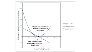
The wage curve for the Beta technique is a straight line. This affine property results from the Organic Composition of Capital being the same in copper production and in corn production, when the Beta technique is adopted. To help visualization, I also graph the difference between the wage curves (Figure 2). The Beta technique is only cost-minimizing at the switch point at the higher rate of profits. The tangency of the wage curves for the Alpha and Beta techniques is manifested in Figure 2 by the non-negativity of the difference in these curves.

|
| Figure 2: Distance Between Wage Curves |
I'm sort of proud of this example. I suppose I could, at least, submit it for publication somewhere. But it is only a side effect of a larger project I guess I am pursuing.
I want to introduce a distinction among fluke switch points. Every bifurcation (that is, a change in the sequence of switch points and cost-minimizing techniques along the wage frontier) is a fluke. Some perturbation of a coefficient of production from a bifurcation value will change that sequence. Suppose a perturbation of a coefficient of production not involved in a bifurcation, in some sense, leaves the qualitative story. One can use the same bifurcation to tell a story about, say, technological progress. This is a generic bifurcation.
Accept, for the sake of argument, that prices of production tell us something about actual prices. The economy is never in an equilibrium, but owners of firms are always interested in increasing their profits. One can never expect observed technology to meet the fluke conditions of a generic bifurcation. But it can tell us something about how the dynamics of income distribution, for example, vary with technological progress.
Suppose one perturbs, in the example, the coefficient of production for the amount of iron needed to produce iron. (I denote this coefficient, in a fairly standard notation, as a1,1β.) Then, either the wage curves for the. Alpha and Beta techniques will not intersect at all or they will intersect twice. In the latter case, one can vary a1,1γ to find an example in which all three wage curves intersect at one or another of the switch points. But the tangency will be lost. So I consider the fluke point illustrated to be a non-generic bifurcation.
Non-generic bifurcations arise in a complete bifurcation analysis. The model illustrated remains open. Income distribution is not specified. Nevertheless, I think this theoretical analysis can say something to those who are attempting to empirically apply the Leontief-Sraffa model.
 Heterodox
