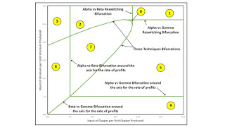
Figure 1: A Blowup of a Bifurcation Diagram1.0 Introduction I have been working on an analysis of structural economic dynamics with a choice of technique. Technical progress can result in a variation in the switch points and the succession of techniques with wage curves on the outer wage frontier. I call such a variation a bifurcation, and I have identified normal forms for four generic bifurcations. This post prevents an example in which all four generic bifurcations appear. 2.0 Technology The example in is one of an economy in which four commodities can be produced. These commodities are called iron, copper, uranium, and corn. The managers of firms know of one process for producing each of the first three commodities. They know of three processes for producing corn. Table 1
Topics:
Robert Vienneau considers the following as important: Example in Mathematical Economics, Sraffa Effects
This could be interesting, too:
Robert Vienneau writes Austrian Capital Theory And Triple-Switching In The Corn-Tractor Model
Robert Vienneau writes Double Fluke Cases For Triple-Switching In The Corn-Tractor Model
Robert Vienneau writes The Emergence of Triple Switching and the Rarity of Reswitching Explained
Robert Vienneau writes Recap For A Triple -Switching Example
|
| Figure 1: A Blowup of a Bifurcation Diagram |
I have been working on an analysis of structural economic dynamics with a choice of technique. Technical progress can result in a variation in the switch points and the succession of techniques with wage curves on the outer wage frontier. I call such a variation a bifurcation, and I have identified normal forms for four generic bifurcations. This post prevents an example in which all four generic bifurcations appear.
2.0 TechnologyThe example in is one of an economy in which four commodities can be produced. These commodities are called iron, copper, uranium, and corn. The managers of firms know of one process for producing each of the first three commodities. They know of three processes for producing corn. Table 1 specifies the inputs required for a unit output for each of these six processes. Each column specifies the inputs needed for the process to produce a unit output of the designated industry. Variations in the parameters a11, β and a11, γ can result in different switch points appearing on the frontier.
| Input | Industry | ||
| Iron | Copper | Uranium | |
| Labor | 1 | 17,328/8,281 | 1 |
| Iron | 1/2 | 0 | 0 |
| Copper | 0 | a11, β | 0 |
| Uranium | 0 | 0 | a11, γ |
| Corn | 0 | 0 | 0 |
Three processes are known for producing corn (Table 2). As usual, these processes exhibit CRS. And each column specifies inputs needed to produce a unit of corn with that process.
| Input | Process | ||
| Alpha | Beta | Gamma | |
| Labor | 1 | 361/91 | 3.63505 |
| Iron | 3 | 0 | 0 |
| Copper | 0 | 1 | 0 |
| Uranium | 0 | 0 | 1.95561 |
| Corn | 0 | 0 | 0 |
Consider the variation in the number and location of switch points as the coefficient of production for the input of copper per unit copper produced, a11, β, falls from over 48/91 to around 1/4. In this analysis, the coefficient of production for the input of uranium per unit uranium produced, a11, γ, is set to 3/5. This variation in a11, β, while all other coefficients of production are fixed, describes a type of technical progress in the copper industry.
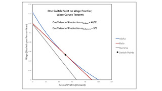
Figure 2 shows the configuration of wage curves near the start of this story. The Gamma technique is never cost-minimizing. For all feasible rates of profits, the wage curve for the Gamma technique falls within the wage frontier. For a parameter value of a11, β of 48/91, the Alpha technique is always cost-minimizing. A single switch point exists, at which the wage curve for the Beta technique is tangent to the wage curve for the Alpha technique, and the Beta technique is also cost-minimizing. I call a configuration of wage curves like that in Figure 2 a reswitching bifurcation. For a slightly lower value of a11, β, two switch points would emerge. The Alpha technique would be cost-minimizing for low and high rates of profits, with the Beta technique cost-minimizing at intermediate rates of profits.
|
| Figure 2: A Reswitching Bifurcation |
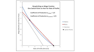
Figure 3 shows the configuration of wage curves when a11, β has fallen to one half. The interval with high rates of profits where the Alpha technique is uniquely cost-minimizing has vanished. The switch point between Alpha and Beta at high rates of profits occurs at a wage of zero. I call Figure 3 an example of a bifurcation around the axis for the rate of profits. For a slightly smaller value of a11, β, the switch point on the axis would vanish, and only one switch point would exist, in this example, for a non-negative wage.
|
| Figure 3: A Bifurcation around the Axis for the Rate of Profits |
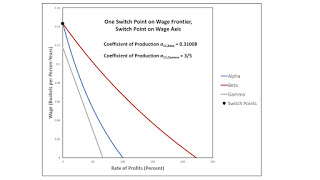
Suppose the coefficient of production a11, β were to fall to approximately 0.31008. Figure 4 shows the resulting configuration of wage curves. The Beta technique is cost-minimizing for all feasible positive rates of profit. A single switch point exists, between Alpha and Beta, on the wage axis. If a11, β were to fall even further, no switch points would exist, and Beta would also be cost-minimizing for a rate of profits of zero. I call this an example of a bifurcation around the wage axis.
|
| Figure 4: A Bifurcation around the Wage Axis |
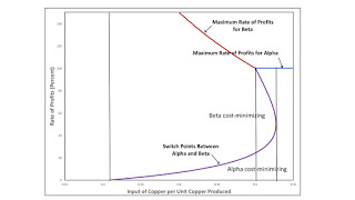
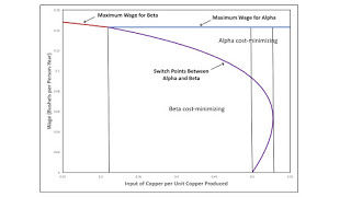
Figures 5 and 6 summarize the above discussion. The coefficient of production a11, β is plotted on the abscissa in each figure. The rates of profits and the wage, respectively, are plotted on the ordinate. Switch points are graphed. The maximum rates of profits for the Alpha and Beta technique are plotted in Figure 5. In Figure 6, the maximum wages for Alpha and Beta are plotted. Each of the three bifurcations in Figure 2, 3, and 4 is shown as a thin vertical line in Figures 5 and 6. The wage curve for the Beta techniques moves outward as one passes from the right to the left in the figures. One can see the single switch point becoming two, and the distance between the two, in terms of either the rate of profits of the wage, becoming greater. The rate of profits for one switch point eventually exceeds the maximum rate of profits and disappears. The rate of profits for the other switch point falls below zero, leaving Beta cost-minimizing for all feasible rates of profits and wages. In short, structural economic dynamics, for the case examined here, can be summarized in either one of these two graphs.
|
| Figure 5: A Bifurcation Diagram for Technical Progress in the Copper Industry |
|
| Figure 6: A Bifurcation Diagram for Technical Progress in the Copper Industry |
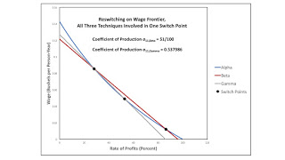
An analysis of technical progress in the uranium industry illustrates another type of bifurcation. Let a11, β be set to 51/100, and let the coefficient of production for the input of uranium per unit uranium produced, a11, γ, fall from around 0.55 to 0.4. Figure 7 shows the configuration of wage curves when a11, γ is approximately 0.537986. The wage curves for Alpha and Beta exhibit reswitching. The wage curve for the Gamma technique also intersects the switch point at the lower rate of profits. I call such a configuration of wage curves a three-technique bifurcation. Aside from the switch point, the Gamma technique is never cost-minimizing.
|
| Figure 7: A Three Technique Bifurcation |
As a11, γ decreases, the wage curve for the Gamma technique moves outward. At an intermediate value, the wage curve for Gamma intersects the wage curves for Alpha and Beta at different switch points. The reswitching example is transformed into one of capital reversing without reswitching.
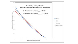
Figure 8 displays a case where the wage curve for Gamma has moved outwards until it intersects the other switch point for the reswitching example. Other than at the switch point, the Beta technique is not cost minimizing for any feasible rate of profits. Figure 8 is also a case of a three-technique bifurcation.
|
| Figure 8: Another Three Technique Bifurcation |
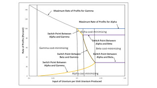
Figure 9 is a bifurcation diagram illustrating this analysis of technical progress in the uranium industry. It graphs the rate of profits against the coefficient of production a11, γ. Switch points on the wage frontier, as well as the maximum rates of profits for the Alpha and Gamma technique, are graphed. The two thin vertical lines toward the right side of the graph are the two three-technique bifurcations. For a slightly lower value of a11, γ than used in Figure 8, this is a reswitching example between Alpha and Gamma. As a11, γ falls even lower, both switch points disappear over the axis for the rate of profits and the wage, respectively, in a graph of wage curves. That is, this example exhibits another illustration of both a bifurcation around the axis for the rate of profits and a bifurcation around the wage axis.
|
| Figure 9: A Bifurcation Diagram for Technical Progress in the Uranium Industry |
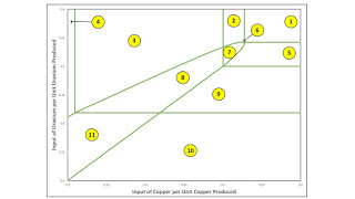
Sections 3.1 and 3.2 each graph switch points against a parameter in the numerical example. A more comprehensive analysis would consider all possible combinations of valid parameter values. One would need to draw a twelve-dimensional space. A part of the space defined by feasible combinations of positive values of a11, β and a11, γ is illustrated in Figure 10, instead Eleven regions are numbered in the figure. Figure 1 enlarges part of Figure 10 and labels the loci dividing regions with specific types of bifurcations.
|
| Figure 10: A Bifurcation Diagram for the Parameter Space |
Each numbered region contains an interior. For points in the interior of a region, a sufficiently small perturbation of the coefficients of production a11, β and a11, γ leaves unchanged the number and pattern of switch points. The sequence of cost-minimizing techniques along the wage frontier between switch points is also invariant within regions. Accordingly, Table 3 lists switch points and cost-minimizing techniques for each region. The techniques are specified in order, from a rate of profits of zero to the maximum rate of profits. In several regions, such as region 2, the same technique is listed more than once, since it appears on the wage frontier in two disjoint intervals. Each locus dividing a pair of regions is a bifurcation. The reader can check that the labels for bifurcations in Figure 1 are consistent with Table 3.
| Region | Techniques | ||
| 1 | Alpha throughout | ||
| 2 | Alpha, Beta, Alpha | ||
| 3 | Alpha, Beta | ||
| 4 | Beta throughout | ||
| 5 | Alpha, Gamma, Alpha | ||
| 6 | Alpha, Gamma, Alpha, Beta, Alpha | ||
| 7 | Alpha, Gamma, Beta, Alpha | ||
| 8 | Alpha, Gamma, Beta | ||
| 9 | Alpha, Gamma | ||
| 10 | Gamma | ||
| 11 | Gamma, Beta | ||
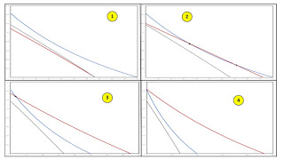
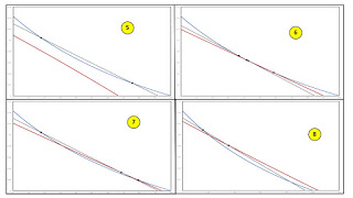
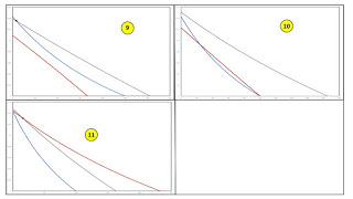
To aid in visualization, Figures 11, 12, and 13 graph wage curves and switch points on the wage frontier for each of the eleven regions. Within a region, the number of and characteristics of intersections of wage curves not on the frontier can vary. For example, the graph for region 8 in the lower right of Figure 12 shows an intersection between the wage curves for the Alpha and Gamma techniques at a high rate of profits. That second intersection between these wage curves can disappear over the axis for the rate of profits while leaving the sequence, if not the location, of cost-minimizing techniques and switch points on the frontier unchanged.
|
| Figure 11: Wage Curves for Regions 1 through 4 |
|
| Figure 12: Wage Curves for Regions 5 through 8 |
|
| Figure 13: Wage Curves for Regions 9 through 11 |
The numerical example is an instance of the Samuelson-Garegnani model. Variations in the two coefficients of production for the copper industry have no effect on the location of intersections between wage curves for Alpha and Gamma. Thus, one obtains the horizontal lines in Figures 1 and 10. Likewise, variations in a11, γ do not affect intersections between the wages curves for Alpha and Beta. This property results in the vertical lines in the bifurcation diagram. Bifurcations in which wage curves for both Beta and Gamma are involved result in the more or less diagonal curves in Figures 1 and 10.
Section 3.1 tells a tale of technical progress in the copper industry. This story is illustrated by the bifurcation diagrams in Figures 1 and 10. The chosen values for a11, β divide regions 1, 2, 3, and 4. Figure 2 lies along the vertical line dividing regions 1 and 2. Figure 3 illustrates the division between regions 2 and 3, and Figure 4 illustrates the corresponding division between regions 3 and 4. The vertical line towards the left side of Figure 10 is a bifurcation across the wage axis.
Similarly, Section 3.2 illustrates bifurcations along a movement downward in Figures 1 and 10. Such a downward movement would pass through regions 2, 7, 5, 9, and 10. Figure 7 illustrates parameters on the locus dividing regions 2 and 7. Figure 8 illustrates the division between regions 7 and 5. The line dividing regions 5 and 9 is a bifurcation around the axis for the rate of profits, and the line dividing regions 9 and 10 is a bifurcation around the wage axis. All four bifurcations are illustrated in Figure 9.
The above partitioning of the parameter space formed by coefficients of production suggests the existence of bifurcations not yet illustrated. For example, a three-technique bifurcation is located anywhere along the locus dividing regions 6 and 7. This bifurcation differs from the three-technique bifurcations illustrated by Figures 7 and 8. Or consider the point that separates regions 1, 2, 5, and 6. The Alpha technique is cost minimizing for all feasible rates of profits for these coefficients of production. Two switch points exist, and at each one of these switch points another technique is tied with the Alpha technique. The wage curve for the Gamma technique is tangent to the wage curve for the Alpha technique at the switch point with the lower rate of profits. The wage curve for the Beta technique is tangent to the wage curve for the alpha technique at the other switch point. The point on the intersection between the loci dividing regions 2, 6, and 7 is interesting. The coefficients of production specified by this point characterize a three-technique bifurcation in which the wage curves for the Alpha and Gamma techniques are tangent at the appropriate switch point. This discussion has not exhausted the possibilities.
 Heterodox
