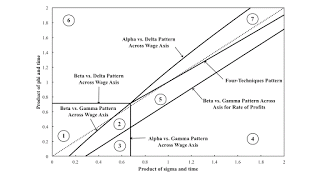
Figure 1: Partition of the Parameter Space1.0 Introduction I here provide some notes on a perturbation of an example from Salvadori and Steedman (1988). Consider an economy in which n commodities are produced in n industries. In each industry, a single commodity is produced from inputs of labor and the services of previously produced capital goods. Suppose the technology can be represented in each industry by a continuously-differentiable production function. The wage-rate of profits frontier for such a model does not contain any switch points. In other words, for each feasible rate of profits, a single technique is cost minimizing. Nevertheless, the cost-minimizing technique varies continuously with the rate of profits. Furthermore, the process associated with the cost-minimizing
Topics:
Robert Vienneau considers the following as important: Example in Mathematical Economics, Sraffa Effects
This could be interesting, too:
Robert Vienneau writes Austrian Capital Theory And Triple-Switching In The Corn-Tractor Model
Robert Vienneau writes Double Fluke Cases For Triple-Switching In The Corn-Tractor Model
Robert Vienneau writes The Emergence of Triple Switching and the Rarity of Reswitching Explained
Robert Vienneau writes Recap For A Triple -Switching Example
|
| Figure 1: Partition of the Parameter Space |
I here provide some notes on a perturbation of an example from Salvadori and Steedman (1988).
Consider an economy in which n commodities are produced in n industries. In each industry, a single commodity is produced from inputs of labor and the services of previously produced capital goods. Suppose the technology can be represented in each industry by a continuously-differentiable production function. The wage-rate of profits frontier for such a model does not contain any switch points. In other words, for each feasible rate of profits, a single technique is cost minimizing. Nevertheless, the cost-minimizing technique varies continuously with the rate of profits. Furthermore, the process associated with the cost-minimizing technique in each industry also varies continuously with the rate of profits.
Suppose, instead, that the processes in each industry were represented by a set of fixed-coefficient processes, instead of a smooth production function. What would hold in a discrete model that is in the spirit of the neoclassical model? I suggest that at each switch point on the frontier, 2n wage curves would intersect. In a model with two produced commodities and two processes available in each industry, four wage curves would intersect at the single switch point. With three produced commodities, eight wage curves would intersect. The natural properties for a neoclassical model - if that is what this is - are flukes to several degrees.
I do not necessarily claim anything revelatory from the details of this post. I am testing the applicability of my pattern analysis by trying it out for various examples. Although you cannot tell from my presentation, the graphs I draw rely less on numerical approximations than in many of my earlier examples. This example is the first I have seen where a pattern with a co-dimension of two or higher happens to form a one-dimensional locus (curved line) in the two-dimensional slice of the parameter space I graph. Salvadori and Steedman could have varied their example in an infinite number of ways and still had an example where all processes varied at a switch point.
2.0 TechnologyI make my usual assumptions about technology. At a given point in time, managers of firms know of a number of production processes (Table 1). A single commodity - a ton iron or a bushel corn in the example - is the output of each process. Each process lasts a year and exhibits constant returns to scale. Inputs are defined in physical units. For example, labor inputs are specified in terms of person-years per ton iron output or per bushel corn output. All inputs are used up in production; there is no fixed capital or joint production.
| Input | Iron Industry | Corn Industry | ||
| (a) | (b) | (c) | (d) | |
| Labor | 1 e1 - σ t | 2 e1 - φ t | 1 | 2 |
| Iron | 0 | 0 | 2/3 | 1/2 |
| Corn | (2/3) e1 - σ t | (1/2) e1 - φ t | 0 | 0 |
To produce a self-sustaining net output with this technology, both iron and corn must be produced. Four techniques can be defined with this technology (Table 2).
| Technique | Processes |
| Alpha | a, c |
| Beta | b, d |
| Gamma | a, d |
| Delta | b, c |
I have defined the technology such that coefficients of production decrease with time in both processes for producing iron. The rate at which they decrease differs between the two processes. A more general case would allow for technical process in each of the processes for producing corn.
3.0 A Temporal PathI first consider the variation with time of prices of production for a special case. Consider:
σ = φ = 1
I make the usual assumptions for prices. Relative spot prices are stationary, such that the same rate of profits is earned in both industries if the technology at a given point of time had prevailed over the year. I assume labor is advanced, and wages are paid out of the surplus at the end of the year. A bushel corn is taken as the numeraire. Supernormal profits cannot be made for either process comprising the chosen technique(s). No process in use incurs extra costs.
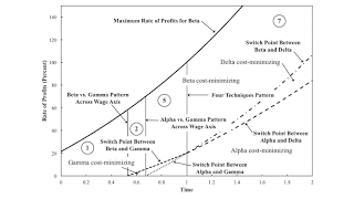
Figure 2 shows how cost-minimizing techniques, the maximum rate of profits, and switch points vary with time. In the region label 1, the Beta technique is cost-minimizing for all feasible rates of profits. The Gamma technique is cost-minimizing for high wages and low rates of profits in Reqion 2. A single switch arises, where wage curves for the Beta and Gamma techniques intersect on the frontier. In the language of the technical terminology I have been introducing, the boundary between Regions 1 and 2 is a pattern across the wage axis. Other patterns are labeled in the diagram.
|
| Figure 2: Variation of Switch Points with Time |
When t = 1, this model reduces to Salvadori and Steedman's example. A single switch exists, with a rate of profits, r0, of 20 percent and a wage of (1/5) bushel per person-year. The wage curves for all four techniques intersect at the switch point. I call the boundary between Regions 5 and 7 a four technique pattern.
I argue that a four technique pattern is of co-dimension two, in my jargon. Each pattern is defined for a switch point. So, in a pattern, at least two wage curves intersect at a switch point:
wα(r0) = wγ(r0)
The co-dimension is the number of additional conditions that must be satisfied for the pattern. Here are two more conditions:
wβ(r0) = wδ(r0)
wα(r0) = wβ(r0)
In this example, for any switch point between the Alpha and Beta techniques, all processes are cost-minimizing. Thus, all techniques are cost-minimizing at such a switch point. For any set of parameters (σ, φ, t) at which there exists a switch point on the frontier between Alpha and Gamma and between Beta and Delta, all techniques are cost-minimizing. In the example, the first two conditions imply the third because of the processes of which the techniques are composed. I think this implication does not hold in general, for all technologies. So I think the definition of a four technique pattern must include three equalities.
4.0 Partition of the Parameter SpaceThe above analysis can be generalized, to consider any combination of (σ t) and (φ t). Figure 1, at the top of the post, partitions the parameter space into seven regions. In any given region, the switch points and the wage curves along the frontier do not vary qualitatively. (Maximum wage, maximum rate of profits, and rate of profits for switch points may vary.) Table 3 lists the switch points and wage curves along the wage frontier, for each region.
| Region | Switch Points | Techniques |
| 1 | None | Beta |
| 2 | Between Beta & Gamma | Gamma, Beta |
| 3 | None | Gamma |
| 4 | Alpha & Gamma | Alpha, Gamma |
| 5 | Alpha & Gamma, Beta & Gamma | Alpha, Gamma, Beta |
| 6 | Beta & Delta | Delta, Beta |
| 7 | Alpha & Delta, Beta& Delta | Alpha, Delta, Beta |
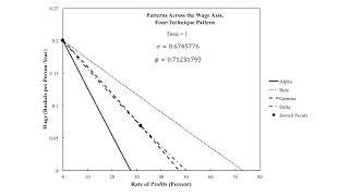
As an aid to visualization, I present some specific configuration of wage curves. Consider the point in the parameter space that is simultaneously on the boundary of Regions 1, 2, 5, 6, and 7. At this point, all techniques are cost-minimizing for a rate of profits of zero. It is simultaneously a four-technique pattern and patterns across the wage axis. Figure 3 shows the wage curves in this case. For feasible positive rates of profits, the Beta technique is uniquely cost-minimizing.
|
| Figure 3: Patterns over the Wage Axis |
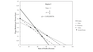
Figure 1 shows loci for three wage patterns intersecting at the point in the parameter space with wage curves illustrated above. Since six pairs of (unordered) techniques can be chosen from four techniques, one might think that six wage patterns should intersect at this point. But I am only defining patterns for switch points on the frontier. To illustrate, consider figure 4, which shows wage curves for a point in Region 5. The wage curves for the Gamma and Delta techniques intersect on the wage axis. Neither, however, are cost-minimizing here; the Alpha technique is cost-minimizing for a rate of profits of zero.
|
| Figure 4: Wage Frontier in Region 5 |
Region 7 is the other region in three techniques are cost-minizing along the wage frontier. Figure 5 illustrates Region 7. For this particular set of parameters, the wage curves for the Gamma and Delta techniques are tangent at a point within the wage frontier. As far as I can tell, no reswitching patterns arise in this example, for switch points on the frontier.
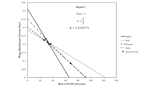
|
| Figure 5: Wage Frontier in Region 7 |
It is also the case that if one extends Figure 1 to the right, the locus for the four-technique pattern never ends. There is not some set of parameter values where the wage curves for all techniques intersect at the maximum rate of profits.
In a perturbation of the example, one can find a set of parameters at which the wage curves for all four techniques intersect at a switch point for a rate of profits of zero. And the parameters can be varied such that the rate of profits for a switch point for all four techniques can be any positive rate of profits.
Reference- Salvadori, Neri and Ian Steedman. 1988. No Reswitching? No Switching! Cambridge Journal of Economics, 12: 481-486.
 Heterodox
