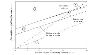
Figure 1: A Two-Dimensional Pattern Diagram1.0 Introduction This post continues this example of the application of pattern analysis to the study of fixed capital. I generalize the technology in the previous post. Technical progress can now proceed at different rates in the production and use of machines. I partition the resulting two-dimensional parameter space based on how the distribution of income, in the system of prices of production, alters the economically efficient length to run the machine. And I find an example in this parameter space that conforms to outdated neoclassical intuition on such matters. 2.0 Technology Table 1 represents the technology for this example. Machines and corn are produced in this economy. Corn is the only consumption good. New machines are produced
Topics:
Robert Vienneau considers the following as important: Example in Mathematical Economics, Joint Production
This could be interesting, too:
Robert Vienneau writes Austrian Capital Theory And Triple-Switching In The Corn-Tractor Model
Robert Vienneau writes Double Fluke Cases For Triple-Switching In The Corn-Tractor Model
Robert Vienneau writes The Emergence of Triple Switching and the Rarity of Reswitching Explained
Robert Vienneau writes Recap For A Triple -Switching Example

|
| Figure 1: A Two-Dimensional Pattern Diagram |
This post continues this example of the application of pattern analysis to the study of fixed capital. I generalize the technology in the previous post. Technical progress can now proceed at different rates in the production and use of machines. I partition the resulting two-dimensional parameter space based on how the distribution of income, in the system of prices of production, alters the economically efficient length to run the machine. And I find an example in this parameter space that conforms to outdated neoclassical intuition on such matters.
2.0 TechnologyTable 1 represents the technology for this example. Machines and corn are produced in this economy. Corn is the only consumption good. New machines are produced from inputs of labor and corn. Corn is produced from inputs of labor, corn, and machines. A machine can be worked for two years. After the end of the first year of its working life, it is known as an old machine. I assume each process requires a year to complete and exhibits constant returns to scale.
| Inputs | Industry | ||
| Machine | Corn | ||
| Labor | a0,1 = (1/10) u(t) | a0,2 = (43/40) v(t) | a0,3 = v(t) |
| Corn | a1,1 = (1/16) u(t) | a1,2 = (1/16) v(t) | a1,3 = (1/4) v(t) |
| New Machines | 0 | 1 | 0 |
| Old Machines | 0 | 0 | 1 |
| Outputs | |||
| Corn | 0 | 1 | 1 |
| New Machines | 1 | 0 | 0 |
| Old Machines | 0 | 1 | 0 |
I model technical progress by constantly decreasing inputs into each process, other than machines:
u(t) = e1 - σ t
v(t) = e1 - φ t
Given values of σ t and φ t, technology is specified.
3.0 Choice of TechniqueFor specified parameters, including σ t and φ t, a system of equations and inequalities is specified such that:
- The rate of profits is determined, given a non-negative wage not exceeding a certain maximum.
- For such a given wage, it is determined whether or not running the machine for one or two years is cost-minimizing.
Which technique - running the machine for one or two years - is cost-minizimizing can vary with mathematical variations in the wage.
Figure 1 partitions the parameter space such that the characteristics of the variations in the choice of technique technique do not vary within each region. Each region is bounded by thick (non-dotted) lines. I do not show a fifth region to the right of the graphed portion of the parameter space. Somewhere before a value of σ t of three, the locus labeled "Pattern over wage axis" curves down to cross the locus labeled "Pattern over axis for rate of profits". In Region 5, the latter locus lies above the former. Table 1 briefly describes the cost-minimizing technique in each region.
| Region | Description |
| 1 | Machine is run for 1 year, for all feasible wages. |
| 2 | Machine is run for 2 years, for low wages; 1 year, for high wages. |
| 3 | Reswitching. Machine is run for 2 years, for low and high wages; 1 year for intermediate wages. |
| 4 | Machine is run for 2 years, for all feasible wages. |
| 5 | Machine is run for 1 year, for low wages; 2 years, for high wages. |
Suppose that technical progress in producing and using machines is steady. That is, σ and φ have some fixed values. Each of the two dotted lines in Figure 1 illustrate a path in logical time for such a thought experiment. The 45 degree line corresponds to the case in which σ and φ are equal. The choice of technique along such a path was illustrated in the previous post.
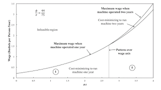
I constructed the dashed line with the smaller slope to pass through Region 5. Technical progress is faster, in this case, in producing machines than in using machines. Figure 2 illustrates this case, which complies with outdated neoclassical intuition. Notice that around the switch point in Region 5, a higher wage is associated with a choice, by managers of firms, to run the machine for a second year. The wage acts like a scarcity index for labor, and the lengths at which firms run machines responds appropriately for a measure of capital intensity. But the example proves that there is no logical necessity for economically efficient decisions to work out like this.

|
| Figure 2: A Pattern Diagram |
This post suggests the tools that I have been developing for post-Sraffian price theory apply, without modification, to models of fixed capital.
 Heterodox
