Figure 1: A Partitioning Of The Parameter Space1.0 Introduction I consider here a case where two different techniques have the same wage curve. A simple labor of theory of value describes prices in the case under consideration. I treat the labor coefficient and another coefficient of production for a process in one technique as parameters. And I look at what happens when they vary. A note on terminology: on the basis of expert advice and peer review, I am no longer using the term "bifurcation" for a pattern of switch points where a perturbation of model parameters, such as coefficients of production, removes or adds a switch point to the wage frontier. Instead, I am calling such a configuration a "pattern." 2.0 Technology Table 1 specifies the technology for this example. I make
Topics:
Robert Vienneau considers the following as important: Example in Mathematical Economics, Sraffa Effects
This could be interesting, too:
Robert Vienneau writes Austrian Capital Theory And Triple-Switching In The Corn-Tractor Model
Robert Vienneau writes Double Fluke Cases For Triple-Switching In The Corn-Tractor Model
Robert Vienneau writes The Emergence of Triple Switching and the Rarity of Reswitching Explained
Robert Vienneau writes Recap For A Triple -Switching Example

|
| Figure 1: A Partitioning Of The Parameter Space |
I consider here a case where two different techniques have the same wage curve. A simple labor of theory of value describes prices in the case under consideration. I treat the labor coefficient and another coefficient of production for a process in one technique as parameters. And I look at what happens when they vary.
A note on terminology: on the basis of expert advice and peer review, I am no longer using the term "bifurcation" for a pattern of switch points where a perturbation of model parameters, such as coefficients of production, removes or adds a switch point to the wage frontier. Instead, I am calling such a configuration a "pattern."
2.0 TechnologyTable 1 specifies the technology for this example. I make the usual assumptions. Each column lists inputs per unit output for each process. Each process exhibits constant returns to scale. Each process requires a year to complete, and there are no joint products. Inputs of capital goods are totally used up in production.
| Input | Iron Industry | Corn Industry | |
| Alpha | Beta | ||
| Labor | (1/8) Person-Yr. | u | (1/2) |
| Iron | (1/2) Ton | v | 2 |
| Corn | (1/16) Bushel | (1/80) | (1/4) |
Two techniques can be created out of these processes. The Alpha technique consists of the iron-producing process labeled Alpha and the corn-producing process. Likewise, the Beta technique consists of the iron-producing process labeled Beta and the corn-producing process.
I think I'll say something about how I created this example. A simple labor theory of value applies to the Alpha technique. The wage curves associated with the Alpha and Beta techniques are identical when u = (1/8) person-year and v = (7/10) ton. This special case is an application of some math I have set out in a working paper.
3.0 PricesI take corn as the numeraire and assume labor is advanced. Wages are paid out of the surplus at the end of year.
3.1 AlphaThe price of production for iron, when the Alpha technique is in use, is:
pα = (1/4)
The wage curve for the Alpha technique is:
wα = (1/2)(1 - 3 r)3.2 Beta
The price of production for iron, when the Beta technique is in use, is:
pβ = [(1 + 120u) + (1 - 40u)r)]/{80[(4u - v)r + (1 + 4u - v)]}
The wage curve for the Beta technique is:
wβ = [(10v - 1)r2 -4(5v + 3)r + (29 - 30v)]3.3 Switch Points/{20[(4u - v)r + (1 + 4u - v)]}
One finds switch points by equating the two wage curves:
wα = wβ
One obtains a quadratic equation in the rate of profits, r:
+ (120 u - 20 v - 1) (rswitch)2+ (80 u - 40 v +18) rswitch+ (-40 u - 20 v + 19) = 0
This equation can be factored:
(r + 1)[(120 u - 20 v - 1)r + (-40 u - 20 v + 19)] = 04.0 Special Cases 4.1 A Continuum of Switch Points
I first want to check the special case u = (1/8) and v = (7/10). Recall, this example was created so that the wage curves for the two techniques would be identical in this case. In this special case, the two coefficients for the second factor of the Left Hand Side of the above quadratic equation reduce to zero. So that equation is identically true for all feasible rates of profits. Every point on the wage frontier is a switch point.
4.2 A Pattern Over the Wage AxisIn this pattern, a switch point exists on the wage frontier for a rate of profits of zero. That is, one must be able to factor out r from the left-hand side of the above quadratic equation. In other words, the constant term for the second factor must be zero. One thereby obtains:
-40 u - 20 v + 19 = 0
Or
v = - 2 u + (19/20)4.3 A Pattern Over the Axis for the Rate of Profits
In this pattern, the wage curves have a switch point at the maximum rate of profits. I did not start with the quadratic equation for this special case. The maximum rate of profits for the Alpha and Beta techniques are equal when the two wage curves are identical. The maximum rate of profits for the Beta technique does not depend on the value of labor coefficients. Thus, the condition for this pattern is:
v = (7/10)
You can check that above condition yields a switch point at a rate of profits of (1/3).
4.4 A Reswitching PatternIn a reswitching pattern, the wage curves for two techniques are tangent at a switch point. For the example in which only two commodities are produced, the quadratic equation obtain by equating the wage curves for two techniques has two repeated roots. In other words, the discriminant for this quadratic equation must be equal to zero. Some algebra gives (some Octave code was useful here):
400 (8 u - 1)2 = 0
Or:
u = (1/8)
If v is not equal to (7/10), the above value of u results at repeated roots for a rate of profits of -1. But I am only considering non-negative rates of profits. Thus, a reswitching pattern does not exist for this example at feasible rates of profits.
5.0 VisualizationI can bring the above observations together with various pictures here.
5.1 Variation of Switch Points with Coefficients of ProductionConsider how the wage frontier varies with v, given a particular parameter value of u. (After reading this section, one might consider how the wage frontier varies with u, given a particular value of v.)
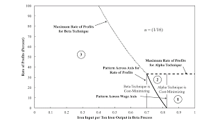
Suppose u is smaller than the special case in which the wage curves for the two techniques are identical for a specific value of v. Figure 2 illustrates this case. In a certain region of variation in v, the wage curves for the Alpha and Beta techniques appear on the frontier, with a single switch point between them.

|
| Figure 2: Variation of v, Case 1 |
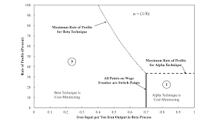
As u increases, towards 1/8, the interval for v in which both wage curves appear on the frontier gets smaller and smaller. Figure 3 shows that, in the limit, this interval narrows to a width of zero. Both wage curves are identical. The wage frontier consists of a continuum of switch points.

|
| Figure 3: Variation of v, Case 2 |
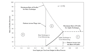
As u increases beyond 1/8, an interval for v once again appears in which the wage frontier contains a single switch point. As shown in Figure 4, the the endpoints of the interval have become interchanged, in some sense.

|
| Figure 4: Variation of v, Case 3 |
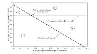
Figure 1, at the top of this post, graphs the parameter space for u and v. The patterns across the wage axis and the over the axis for the rate of profits divide the parameter space into the four numbered regions. Table 2 lists the switch points and the techniques along the wage frontier, in each region, in order of an increasing rate of profits.
| Region | Switch Points | Techniques |
| 1 | None | Alpha |
| 2 | One | Beta, Alpha |
| 3 | None | Beta |
| 4 | One | Alpha, Beta |
My methods for pattern analysis and visualization apply in this case generalizing an instance in which two techniques have identical wage curves.
6.0 ConclusionsI have conjectured that four types of patterns of co-dimension one exist (the three-technique pattern, the pattern over the wage axis, the pattern over the axis for the rate of profits, and the reswitching pattern). This example of two techniques having identical wage curves is not a counter-example to this conjecture. It is simultaneously a a pattern over the wage curve and a pattern over the axis for the rate of profits. Thus, it is at least of co-dimension two.
The conditions for those two patterns, however, are not sufficient for this pattern. They are merely necessary. One could have two wage curves with switch points on the wage axis and on the axis for the rate of profits, but differing for all positive rate of profits less than the maximum rate of profits. The example does make me wonder about my distinction between local and global patterns; this is not the type of global pattern I had in mind when I came up with the idea. And what is the co-dimension for this pattern? Is it of an uncountably infinite co-dimension?
I can see why some might think my write-up is not all that exciting. Likewise, there is a certain amount of tedium in performing the analysis documented above. Nevertheless, I was intrigued to find the above picture emerging. I think I have stumbled upon a vast unexplored landscape in which complicated fluke cases can fit.
 Heterodox
