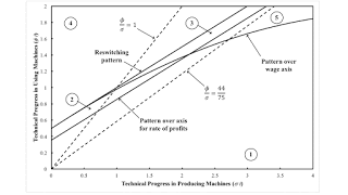
Figure 1: A Partition of a Parameter Space for the Schefold Example1.0 Introduction I want to revisit a perturbation analysis of an example, from Bertram Schefold, of reswitching with fixed capital. Suppose workers use a machine to produce something or other, where the machine lasts several production periods. It is a possible choice to run the machine for less than its full physical life. One might think than choosing to adopt a technique with a longer economic life of the machine is, in some sense, more capital-intensive than choosing to junk it sooner. And this will lead to more output per worker. But, I am surprised to say, this is just not so. The underlying vision of Austrian-school economists is wrong even here. If I worked through all the problems, with full understanding
Topics:
Robert Vienneau considers the following as important: Austrian School Of Economics, Example in Mathematical Economics, Joint Production, Sraffa Effects
This could be interesting, too:
Robert Vienneau writes Austrian Capital Theory And Triple-Switching In The Corn-Tractor Model
Robert Vienneau writes Double Fluke Cases For Triple-Switching In The Corn-Tractor Model
Robert Vienneau writes The Emergence of Triple Switching and the Rarity of Reswitching Explained
Robert Vienneau writes Recap For A Triple -Switching Example
|
| Figure 1: A Partition of a Parameter Space for the Schefold Example |
I want to revisit a perturbation analysis of an example, from Bertram Schefold, of reswitching with fixed capital.
Suppose workers use a machine to produce something or other, where the machine lasts several production periods. It is a possible choice to run the machine for less than its full physical life. One might think than choosing to adopt a technique with a longer economic life of the machine is, in some sense, more capital-intensive than choosing to junk it sooner. And this will lead to more output per worker. But, I am surprised to say, this is just not so. The underlying vision of Austrian-school economists is wrong even here.
If I worked through all the problems, with full understanding of their implications, in Kurz and Salvadori (1995), I would probably already know this. But, at least, I can make this point by examining perturbations of a single numeric example.
2. TechnologyTable 1 shows the coefficients of production for the three processes comprising the available technology. Inputs must be available at the beginning of the year, and outputs become available at the harvest at the end. In the first process, labor uses inputs of corn to produce a new machine. That machine is used by labor in the second process, with inputs of seed corn, to produce more corn and a one-year old machine. In the third process, labor uses inputs of seed corn and the one-year old machine to produce corn. (I did think of calling the machine a "tractor".) The machine varies in physical efficiency over the course of its lifetime. In its second year, it requires less labor to tend it, but more inputs of corn.
| Input | Process | ||
| (I) | (II) | (III) | |
| Labor | (1/10) e1 - σ t | (43/40) e1 - φ t | e1 - φ t |
| Corn | (1/16) e1 - σ t | (1/16) e1 - φ t | (1/4) e1 - φ t |
| New Machines | 0 | 1 | 0 |
| Old Machines | 0 | 0 | 1 |
| Outputs | |||
| Corn | 0 | 1 | 1 |
| New Machines | 1 | 0 | 0 |
| Old Machines | 0 | 1 | 0 |
I postulate the possibility of technical progress. The parameter σ specifies the rate of technical progress in using machines, while φ specifies the rate of technical progress in using machines to produce corn. When (σ t) and (φ t) are unity, this is a reswitching example from Bertram Schefold (1980: 179). Corn is assumed to be the only consumer good, and it also is used as circulating capital. I also take a unit of corn as the numeraire.
A choice of technique arises. I call Alpha the technique in which the machine is operated only one year, and I assume free disposal. Beta is the technique in which the machine is operated for its full physical life time.
3.0 Price EquationsI take corn as numeraire. Although I do not make use of this generality in this post, I formulate systems of equalities and inequalities for prices of production with the possibility of persistent differences in the rate of profits among processes. p1 is the price of a new machine, p2 is the price of an old machine, w is the wage, and r is the scale factor for the rate of profits. The relative rates of profits are specified by given ratios s1, s2, and s3 for the processes, which I take to be unity throughout. Coefficients of production are taken as given; one might think of the parameter t as expressing a very slow, secular time. With these parameters, and either the wage or the scale factor for the rate of profits taken as given, one solves for the prices of new and old machines, the other distributive variable, and the choice of technique.
3.1 Price Equations for the Alpha TechniqueSuppose the Alpha technique is cost-minimizing, and the machine is discarded after being used for one year. The price of a new machine, the wage, and the scale factor for the rate of profits are related by the following two equations:
[(1/16) e1 - σ t](1 + s1r) + [(1/10) e1 - σ t] w = p1
[(1/16) e1 - φ t + p1](1 + s2r) + [(43/40) e1 - φ t] w = 1
The first equations comes from the process for producing a new machine. The second equation comes from the process for producing corn with a new machine. The price of an old machine is zero:
p2 = 0
For the Alpha technique to be cost-minimizing, extra profits must not be available from operating the process that produces corn with an old machine. That is, the cost of a unit level operation of that process must not fall below revenues:
[(1/4) e1 - φ t](1 + s3r) + [e1 - φ t] w ≥ 1
A switch point exists when the above equation is met with equality.
3.2 Price Equations for the Beta TechniqueNow suppose the Beta technique is cost-minimizing. The prices of a new and old machine, the wage, and the scale factor for the rate of profits are related by three equations:
[(1/16) e1 - σ t](1 + s1r) + [(1/10) e1 - σ t] w = p1
[(1/16) e1 - φ t + p1](1 + s2r) + [(43/40) e1 - φ t] w = 1 + p2
[(1/4) e1 - φ t + p2](1 + s3r) + [e1 - φ t] w = 1
For the Beta technique to be cost-minimizing, the price of an old machine must not be negative.
p2 ≥ 0
Here, too, a switch point exists when the above equation is met with equality. Suppose prices of production for the Beta technique yield a negative price for an old machine. This is a signal to firms that they should truncate the economic life of the machine. They should only operate it for one year.
4.0 PerturbationsI do my usual thing of analyzing how the choice of technique varies with technical progress along a secular path, given values of parameters that specify the rate of decrease in specified coefficients of production. Technical progress in the example reduces the inputs of labor and circulating capital needed to produce a given output. The notation allows the rate of technical progress to differ between the machine and corn industries. The rate of technical progress is assumed to affect both processes that produce corn in the same way, whether or not the machine the workers use is new or old.
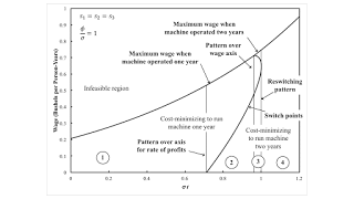
4.1 A Temporal PathThe choice of technique varies with distribution and technical progress. Figure 2 illustrates one particular ratio of the rate of technical progress in producing machines to the rate in using machines. Changes in the number and characteristics of switch points occur with patterns already described in previous blog posts. Switch points appear over the axis for the rate of profits and over the wage axis. Schefold's particular parameterization occurs just before switch points vanish in a reswitching pattern.
|
| Figure 2: A Case of Variation in Switch Points with Technical Progress |
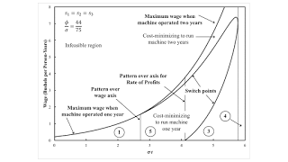
Figure 3 illustrates another particular ratio of the rate of technical progress in producing machines to the rate in using machines. Here too, the technical progress in using machines overwhelms technical progress in producing machines, and this is manifested by a transition ultimately from a region in which the economic life of a machine is one year to a region in which its economic life is its whole physical life, whatever the distribution of income. In this example of technical progress, a pattern over the wage axis precedes a pattern over the axis for the rate of profits. A reswitching example arises and disappears. It is then cost-minimizing to run the machine for its full physical life at high and low wages, but at intermediate wages cost-minimizing firms will truncate the economic life of the machine.
|
| Figure 3: Another Case of Variation in Switch Points with Technical Progress |
At each point on the two paths through logical time characterized by Figures 2 and 3, the amount of technical progress in producing machines and in using machines is specified. Figure 1 partitions the resulting parameter space, based, as usual, on the number and characteristics of switch points in the choice of technique. Table 2 notes the switch points and lists the cost-minimizing technique, from a low to a high wage, for each numbered region. The locii separating Regions 1 and 2 and Regions 3 and 4 are parallel affine functions. The locus for the reswitching pattern is tangent to the locus for the pattern over the wage axis at the intersection of Regions 2, 3, and 4. Figure 1 demonstrates the applicability of the taxonomy of fluke switch points to the case of fixed capital.
| Region | Switch Points | Cost-Minimizing Techniques |
| 1 | None | Alpha |
| 2 | One | Beta, Alpha |
| 3 | Two | Beta, Alpha, Beta |
| 4 | None | Beta |
| 5 | One | Alpha, Beta |
The Schefold example is in narrow edge at the left of Region 3, along the dotted line corresponding to Figure 2. Just as this approach of partitioning (projections of) parameter spaces can be used to construct fluke switch points, it can also be used to improve examples of non-fluke switch points. Other parameters in Region 3 can result in switch points further apart on the wage frontier. The price of an old machine, at prices of production for the Beta technique, can be more noticeably negative when the Alpha technique is cost-minimizing.
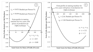
5.0 Compare and Contrast Regions 2 and 5Comparing and contrasting the single switch point in Regions 2 and 5 is interesting. Figures 4 and 5 illustrate the application of the direct method to analyze the choice of technique. When the machine is junked after one year, the price of an old machine is zero. Figure 4 shows extra profits in operating the machine for the second year with prices of production in this case. Around the switch point in Region 2, it pays to run the machine for a second year for higher rates of profits. On the other hand, around the switch point in Region 5, it pays to run the machine for the second year at lower rates of profits. Figure 5 shows the price of the old machine, given prices of production, when the machine is run for two years. A negative price shows that the cost-minimizing firm should truncate the economic life of machine to one year. Both figures yield the same conclusion about the choice of technique in the two regions. (This consistency is guaranteed in a pure fixed capital example with no superimposed joint production.)
|
| Figure 4: Regions 2 and 5 with Price of Old Machine of Zero |
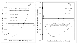
|
| Figure 5: Price of Production when Machine Runs for Two Years |
Around the switch points in both Regions 2 and 5, a lower wage is associated with cost-minimizing firms wanting to hire more labor, given net output (Table 3). As one might expect, the adoption of a more labor-intensive technique is associated with lower net output per worker. It seems that the economic life of a machine cannot be mapped to the capital-intensity of a technique. Adopting a technique in which a machine is run longer is not necessarily more capital-intensive in that it does not necessarily raise output per worker for the economy as a whole. This counter-intuitive result, at least by traditional neoclassical and Austrian teaching, obtains in Region 2.
| Region 2 | Region 5 | |
| Economic Life of Machine | Run for two years at higher rate of profits | Run for one year at higher rate of profits |
| Consumption per Person-Year | Decreased at higher rates of profits | Decreased at higher rate of profits |
| Employment, given net corn output | Increased at lower wage | Increased at lower wage |
Unambiguous physical measures are available here for examining central claims in Austrian capital theory. Net output in a stationary state in this model consists of a single consumption good, and labor is taken as homogeneous. Around a switch point exhibiting capital-reversing, a lower interest rate is associated with the adoption of a technique that produces less net output per unit of labor time. If a financial measure of capital intensity is adopted such that, around all switch points, lower interest rates are associated with the use of a technique with a longer average period of production, the association between more roundabout methods of production and greater productivity is broken. Austrian capital theory and Austrian business cycle theory fails to be sustained
In a model of fixed capital with only a single machine in use, the number of production cycles for the economic life of the machine is an unambiguous measure of roundaboutness. The numerical example in this chapter reveal that no connection necessarily exists between lower interest rates and the extension of the economic life of a machine. The example in Region 3 is a reswitching example. Necessarily, in a reswitching example in a model of fixed capital, a lower rate of profits is associated, around one of the switch points, with the truncation of the economic life of the machine.
The Austrian theory of capital is also refuted in Region 2 in the example, even with a single switch point. Around the switch point, a lower rate of profits is associated with a truncation of the economic life of a machine, not the extension of how long this machine is used in production cycles. And that truncation is associated with a more capital-intensive technique, as is seen in an increase in net output per worker. These examples demonstrate that the underlying vision behind the Austrian story is simply incorrect. Attempts to evade this proof by adopting a financial definition of capital simply ignore the points at issue.
 Heterodox
