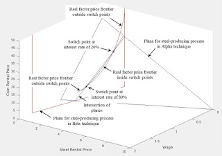
Figure 1: Real Factor Price Frontier1.0 Introduction Carlo Milana has proposed a new way of visualizing the choice of technique, including in the case of reswitching. This way of describing what he has done is not neccessarily how he thinks of it. In this post, I describe his approach with a reswitching example, in a model of the production of commodities by means of commodities. 2.0 Technology Table 1 shows the coefficients of production for this example. Coefficients of production specify inputs per unit output. Each process takes a year to complete. Inputs are totally used up in the production of the outputs. (This example is taken from one of my papers.) Table 1: Coefficients of Production for The Technology InputSteel IndustryCorn IndustryAlphaBetaLabor1275/4641
Topics:
Robert Vienneau considers the following as important: Example in Mathematical Economics, Sraffa Effects
This could be interesting, too:
Robert Vienneau writes Austrian Capital Theory And Triple-Switching In The Corn-Tractor Model
Robert Vienneau writes Double Fluke Cases For Triple-Switching In The Corn-Tractor Model
Robert Vienneau writes The Emergence of Triple Switching and the Rarity of Reswitching Explained
Robert Vienneau writes Recap For A Triple -Switching Example

|
| Figure 1: Real Factor Price Frontier |
Carlo Milana has proposed a new way of visualizing the choice of technique, including in the case of reswitching. This way of describing what he has done is not neccessarily how he thinks of it. In this post, I describe his approach with a reswitching example, in a model of the production of commodities by means of commodities.
2.0 TechnologyTable 1 shows the coefficients of production for this example. Coefficients of production specify inputs per unit output. Each process takes a year to complete. Inputs are totally used up in the production of the outputs. (This example is taken from one of my papers.)
| Input | Steel Industry | Corn Industry | |
| Alpha | Beta | ||
| Labor | 1 | 275/464 | 1 Person-Yr |
| Steel | 1/10 | 113/232 | 2 Tons |
| Corn | 1/40 | 0 | (2/5) Bushels |
Two techniques of production arise in this example. The Alpha technique consists of the Alpha process for producing steel and the corn-producing process. Both steel and corn are basic commodities, in the sense of Sraffa, for the Alpha technique. The Beta technique consists of the Beta process for producing steel and the corn-producing process. Only steel is a Sraffa-basic commodity for the Beta process. Suppose, however, corn is the only consumption good in this example. Then in the Beta technique, as with the Alpha technique, both steel and corn will be (re)produced for both techniques.
3.0 Prices of ProductionIf the Alpha technique is in use in a long-period position, prices satisfy the following two equations:
((1/10) pα,1 + (1/40) pα,2)(1 + r) + wα = pα,1
(2 pα,1 + (2/5) pα,2)(1 + r) + wα = pα,2
Prices are spot prices. The services of produced inputs are paid for at the start of the year, while wages are paid out of the surplus at the end of the year.
The corresponding equations for prices for the Beta technique are:
((113/232) pβ,1)(1 + r) + (275/464) wβ = pβ,1
(2 pβ,1 + (2/5) pβ,2)(1 + r) + wβ = pβ,2
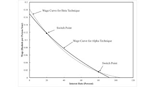
At this point, I take a bushel corn as the numeraire. One can solve the Alpha system of equations, for example, to find (wα/pα,1) as a function of the interest rate. This is the wage curve for the Alpha technique and is shown below. The wage curve for the Beta technique is also graphed. The outer envelope of these curves, called the wage frontier, shows which technique is cost-minimizing at any given interest rate. Both techniques are cost-minimizing at the switch points, which arise for interest rates of 20 percent and 80 percent. Between the switch points, the Alpha technique is cost-minimizing. Outside the switch points, the Beta technique is cost minimizing.

|
| Figure 2: Wage Curves and the Wage Frontier |
In marginalism, the choice of technique is often analyzed in terms of rental prices for factors of production. One can think of the example in terms of three factors: labor, steel, and corn. Steel and corn are capital goods.
Since a choice of production processes arises in the steel industry, I here take steel as numeraire. The rental price, also known as the factor price, for labor is the real wage:
wα,L = wα/pα,1
The rental or factor price for steel is the cost of a the services of a ton of steel when paid at the end of the year:
wα,Steel = pα,1(1 + r)/pα,1
Likewise, the rental or factor price of corn is:
wα,Corn = pα,2(1 + r)/pα,1
Using these definitions, the condition that, when in use, no extra profits are made and no extra costs are in incurred in producing steel with the Alpha process yields the following equation:
(1/10) wα,Steel + (1/40) wα,Corn + wα,L = 1
Notice that this is a linear equation in three variables. It is illustrated by the blue plane in Figure 1. The factor prices for the Beta process yield another linear equation:
((113/232) wβ,Steel + (275/464) wα,L = 1
The plane for Beta is shown in red in Figure 1.
At a switch point, both the Alpha and the Beta processes are eligible for adoption by cost-minimizing managers of firms. Accordingly, switch points must lie on the intersection of the two planes described above. The intersection, although difficult to see, is shown in black in the figure.
In discussing rental or factor prices, I have yet to take into account that corn must also be produced. If one substitutes, on the right-hand side in the three equations defining rental prices, the solution of the Alpha system of equations in Section 3, one obtains factor prices as a parametric function of the interest rate. This is the real factor price curve for the Alpha technique and is shown in blue above. The real factor price curve for the Beta technique, in red, is easier to see. (Each real factor price curve lies within the plane of the same color.) For each curve, when it lies on the real factor price frontier is indicated. And the switch points do indeed lie on the intersections of the real factor price curves.
5.0 ConclusionDoes the real factor price frontier in Figure 1 provide a mechanism for analyzing the choice of technique? Is the factor price curve for the cost-minimizing technique always furtherest from the origin?
The wage frontier, where applicable, can be drawn in a two-dimensional diagram for examples with any number produced of produced commodities. If n commodities are produced, Milana's diagram illustrates, roughly, the intersections of hyperplanes of dimension (n - 1). And those intersections will be themselves hyperplanes of dimension (n - 2). Switch points, if any, lie in those intersections. The factor price curves will still be one-dimensional curves, as I understand it, in the appropriate hyperplanes.
Obviously, this cannot be visualized in higher dimensions. Nevertheless, the mathematics still works out. Different valid approaches to finding the cost-minimizing technique in a long-period position, given an exogenous specification of the distribution of income, in some sense, will all yield the same answer. That is the case for the reswitching example presented here.
 Heterodox
