Figure 1: Two Dimensional Pattern Diagram1.0 Introduction This post extends an example from Bertram Schefold. It presents markup pricing in an example with a machine that can be operated for two years or junked after one year. This is a case of joint production in which, unlike in some cases, the choice of technique can still be analyzed by the construction of the wage frontier. Also, I do not think the question of requirements for use enter in here, and all matrices are square. As usual, this is a proof that "the marginal productivity theory of distribution" (and the neoclassical theory of supply and demand) "is all bosh" (Robinson 1961). 2.0 Technology Table 1 shows the coefficients of production for the three processes comprising the available technology. Inputs must be available
Topics:
Robert Vienneau considers the following as important: Example in Mathematical Economics, Full Cost Prices, Joint Production, Sraffa Effects
This could be interesting, too:
Robert Vienneau writes Austrian Capital Theory And Triple-Switching In The Corn-Tractor Model
Robert Vienneau writes Double Fluke Cases For Triple-Switching In The Corn-Tractor Model
Robert Vienneau writes The Emergence of Triple Switching and the Rarity of Reswitching Explained
Robert Vienneau writes Recap For A Triple -Switching Example

|
| Figure 1: Two Dimensional Pattern Diagram |
This post extends an example from Bertram Schefold. It presents markup pricing in an example with a machine that can be operated for two years or junked after one year. This is a case of joint production in which, unlike in some cases, the choice of technique can still be analyzed by the construction of the wage frontier. Also, I do not think the question of requirements for use enter in here, and all matrices are square. As usual, this is a proof that "the marginal productivity theory of distribution" (and the neoclassical theory of supply and demand) "is all bosh" (Robinson 1961).
2.0 TechnologyTable 1 shows the coefficients of production for the three processes comprising the available technology. Inputs must be available at the beginning of the year, and outputs become available at the harvest at the end. In the first process, labor uses inputs of corn to produce a new machine. That machine is used by labor in the second process, with inputs of seed corn, to produce more corn and a one-year old machine. In the third process, labor uses inputs of seed corn and the one-year old machine to produce corn. (I did think of calling the machine a "tractor".) The machine varies in physical efficiency over the course of its lifetime.
| Input | Machine Industry | Corn Industry | |
| One Process | Another Process | ||
| Labor | a0, 1 = 1/10 | a0, 2 = 43/40 | a0, 3 = 1 |
| Corn | a1, 1 = 1/16 | a1, 2 = 1/16 | a1, 3 = 1/4 |
| New Machines | a2, 1 = 0 | a2, 2 = 1 | a2, 3 = 0 |
| Old Machines | a3, 1 = 0 | a3, 2 = 0 | a3, 3 = 1 |
| Output | |||
| Corn | b1, 1 = 0 | b1, 2 = 1 | b1, 3 = 1 |
| New Machines | b2, 1 = 1 | b2, 2 = 0 | b2, 3 = 0 |
| Old Machines | b3, 1 = 0 | b3, 2 = 1 | b3, 3 = 0 |
The technology is summarized by a row vector a0, the input vector A, and the output vector B. The example satisfies various assumptions that show the economy hangs together, in some sense, and that it is more than viable.
The technology also presents a choice of technique. Managers of firms in corn-production may want to truncate the use of the machine to one year, given certain configurations of prices. In the Alpha technique, the machine is used for two years. I call the technique in which the machine is only used for one year the Beta technique.
3.0 Prices of ProductionThe price equations for the Alpha technique are:
p A (I + r S) + w a0 = p B
where p is a row vector of three prices (the price of corn, the price of a new machine, and the price of a one-year old machine), w is the wage, and r is the scale factor for the rate of profits. In a common notation, I is the identity matrix. The square matrix S is a diagonal matrix. Its diagonal elements express persistent differences in the rate of profits among processes or industries. The rate of profits in the jth process is r sj.
I take corn as the numeraire. This can be expressed as:
p e1 = 1
where e1 is the first column of the identity matrix.
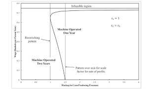
4.0 Some Visualizations of the SolutionAssume, without loss of generality, that the markup coefficient, s1, in the process producing new machines is unity. Figure 2 shows how the choice of technique varies with the wage in the case where the markup coefficients in corn-producing processes do not vary with the age of the machine. When barriers to entry in producing new machines ensure that the markups in corn production fall appreciably below the overall rate of profits, managers of corn-producing firms will operate the machine for its full physical life, whatever the wage. On the other hand, roughly, if the corn-producing industry maintains barrier to entries, the machine will be operated for its full life only at low and high wages. At intermediate wages, the use of the machine will be truncated after one year. As still higher markups in corn-production, the machine will only be operated for the full two years for high wages.

|
| Figure 2: A Pattern Diagram |
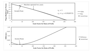
Figure 2 can be constructed in two ways. One is by constructing the wage frontier out of the wage curves for the two techniques. Figure 3 shows an example. This case is for what I call a reswitching pattern. The two wage curves are tangent at the single switch point. In finding the wage curve for the Alpha technique, one can also solve for the price of a one-year old machine. In the analysis of truncation with fixed capital, the machine is operated for only one year when this price turns negative. Switch points between the two techniques arise for wages in which the price of a one-year old machine is zero. I believe this analysis applies with the formulation of markup pricing in this post.

|
| Figure 3: Wage Curves for a Reswitching Pattern |
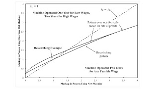
Figure 1, at the top of this post, generalizes the analysis to all values of the markups in the corn-producing processes. Regions are indicated in which the machine is operated for two years, whatever the wage; in which this is an example of reswitching; and in which the machine is operated for two years only for high wages. The dashed (45-degree) line shows the case in which the markup is the same in both corn-producing processes.
I wonder if it makes any economic sense to consider cases off the 45-degree line in Figure 1. In this simple example, the two corn-producing processes are in the same industry, in some sense. If one agrees with this limitation for economic sense, a question arises. How, in some formulation of markup pricing, should such constraints be formulated, in general, for prices of production in models of joint production? Could markups, for instance, vary between the production of mainly wool and mainly mutton? Since definitions of even basic commodities vary among analyses of joint production, I do not see how to identify such processes in general where you might want to raise the question. Maybe these questions could be partly addressed by considering the process of vertical integration.
5.0 ConclusionsThis post has illustrated that the analysis of the choice of technique must be performed in models with fixed capital. Managers of firms always have the choice of truncation, of adopting a technique in which the economic life of a machine is shorter than its physical life. This presents a challenge to attempts to justify Marx's theory of value with Sraffa's standard commodity. I have not even gone into some of the complications raised by pure joint production and models in which multiple types of machines are used.
References- Luigi L. Pasinetti (ed.) 1980. Essays on the Theory of Joint Production. New York: Columbia University Press.
- Joan Robinson. 1961. Prelude to a critique of economic theory. Prelude to a critique of economic theory 13: 53-58.
- Bertram Schefold. 1980. Fixed capital as a joint product and the analysis of accumulation with different forms of technical progress. In Pasinetti 1980.
 Heterodox
