Figure 1: A Partition of a Slice of the Parameter Space1.0 Introduction This post tells a story in which owners of a certain type of land find the amount of their land needed to produce net output declines. Wages stay constant, and the rent for some landlords increases. This example is generalized from Woods (1990). 2.0 Technology This an example (Table 1) of a capitalist economy in which two commodities, iron and corn, are produced. One process is known for producing iron. In the iron industry, workers use inputs of corn to produce an output of iron. Three processes are known for producing corn. Each corn-producing process operates on a specific type of land. These processes can be thought of as examples of joint production. Their outputs are corn and the same quantity of land used
Topics:
Robert Vienneau considers the following as important: Example in Mathematical Economics, Joint Production, Sraffa Effects
This could be interesting, too:
Robert Vienneau writes Austrian Capital Theory And Triple-Switching In The Corn-Tractor Model
Robert Vienneau writes Double Fluke Cases For Triple-Switching In The Corn-Tractor Model
Robert Vienneau writes The Emergence of Triple Switching and the Rarity of Reswitching Explained
Robert Vienneau writes Recap For A Triple -Switching Example
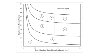
| Figure 1: A Partition of a Slice of the Parameter Space |
This post tells a story in which owners of a certain type of land find the amount of their land needed to produce net output declines. Wages stay constant, and the rent for some landlords increases. This example is generalized from Woods (1990).
2.0 TechnologyThis an example (Table 1) of a capitalist economy in which two commodities, iron and corn, are produced. One process is known for producing iron. In the iron industry, workers use inputs of corn to produce an output of iron. Three processes are known for producing corn. Each corn-producing process operates on a specific type of land. These processes can be thought of as examples of joint production. Their outputs are corn and the same quantity of land used as input, unchanged by the production process. Presumably, some of the labor in these processes is used to maintin the land in a given state.
| Input | Iron Industry | Corn Industry | ||
| I | II | III | IV | |
| Labor | a0,1 = 1 | a0,2 = 1/2 | a0,3 = 3 | a0,4 = 1 |
| Type 1 Land | 0 | b1,2 = 1 | 0 | 0 |
| Type 2 Land | 0 | 0 | b2,3 = 1 | 0 |
| Type 3 Land | 0 | 0 | 0 | b3,4 |
| Iron | a1,1 = 0 | a1,2 = 1/2 | a1,3 = 1/8 | a1,4 = 1/10 |
| Corn | a2,1 = 1/2 | a2,2 = 0 | a2,3 = 0 | a2,4 = 0 |
The specification of technology is completed by noting the values of parameters for the quantities available of non-produced means of production. For this numerical example, let there be T1 = 100 acres of type 1 land, T2 = 80 acres of type 2 land, and T3 = 40 acres of type 3 land. Each process exhibits constant returns to scale, up to the limit imposed by the given quantities of the types of land.
I consider stationary states with a net output consisting solely of corn. A bushel corn is the numeraire. Table 2 lists the possible techniques, along with the range of person-years employment consistent with each technique. The process for producing iron is part of each technique. Table 2 specifies which types of land are fully or partially farmed in each technique.
| Technique | Type of Land | Labor Force | |||
| Type 1 | Type 2 | Type 3 | Min | Maximum | |
| Alpha | Fully farmed | Fully farmed | Partially farmed | 350 | 350 + (44/b3,4) |
| Beta | Partially farmed | Fully farmed | Fully farmed | 250 + (44/b3,4) | 350 + (44/b3,4) |
| Gamma | Fully farmed | Partially farmed | Fully farmed | 100 + (44/b3,4) | 350 + (44/b3,4) |
| Delta | Fully farmed | Partially farmed | Fallow | 100 | 350 |
| Epsilon | Fully farmed | Fallow | Partially farmed | 100 | 100 + (44/b3,4) |
| Zeta | Partially farmed | Fully farmed | Fallow | 250 | 350 |
| Eta | Fallow | Fully farmed | Partially farmed | 250 | 250 + (44/b3,4) |
| Theta | Partially farmed | Fallow | Fully farmed | 44/b3,4 | 100 + (44/b3,4) |
| Iota | Fallow | Partially farmed | Fully farmed | 44/b3,4 | 250 + (44/b3,4) |
| Kappaa | Partially farmed | Fallow | Fallow | 0 | 100 |
| Lambda | Fallow | Partially farmed | Fallow | 0 | 250 |
| Mu | Fallow | Fallow | Partially farmed | 0 | 44/b3,4 |
I might as well step through arithmetic for one of these techniques to illustrate how to find the range of employment compatible with it. Consider Lambda, in which type 2 land is partially farmed. When this type of land is totally farmed, process III is operated at the level of T2/b2,3. The quotient of 80 acres and 1 acre per bushels is 80 bushels, the maximum gross quantity of corn that can be produced with this technique. The amount of iron required as input into process III at this level is a2,3q3, or the product of 80 bushels and 1/8 tons per bushel, that is 10 tons. Producing 10 tons iron requires an input of a2,1q1 = (1/2) 10 = 5 bushels, leaving a net output of 75 bushels for the economy as a whole. The maximum level of employment with the Lambda technique is a0,1q1 + a0,3q3, that is, 1 x 10 + 3 x 80 or 250 person-years. In a stationary state, the level of consumption is 75/250 = 3/10 bushels per person-year.
3.0 Prices of ProductionEach of the four processes yields an equation for the system of prices of production. These equations are:
(1/2)(1 + r) + w = p
(1/2) p (1 + r) + ρ1 + (1/2) w = 1
(1/8) p (1 + r) + ρ2 + 3 w = 1
(1/10) p (1 + r) + b3, 4 ρ3 + w = 1
The variables are:
- p: The price of iron (bushels per ton)
- w: The wage (bushels per person-year).
- r: The rate of profits.
- ρj, j = 1, 2, 3: Rent for type j land (bushels per acre).
All must be non-negative. The left-hand sides shows the cost of operating the process, including the rate of profits on capital goods. Profits, rent, and wages are paid out at the end of the year. The right-hand sides of these equations show the revenues obtained by operating each process at a unit level. For prices of production, the revenues obtained, for operated processes, just cover costs. Costs exceed revenues for non-operated process.
In this model of extensive rent, a final equation must be satisfied by the rents:
ρ1 ρ2 ρ3 = 0
This equation states that the rent on at least one type of land is zero.
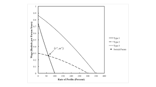
4.0 The Order of Fertility and the Order of RentabilityLand of a type that is left uncultivated, either partially of fully, is in excess supply and pays no rent. Three possibilities for the price system arise. Suppose type 1 land has a rent of zero (ρ1 = 0). Then the first two equations form a system in three variables: the price of iron, the wage, and the rate of profits. They have one degree of freedom in their solution. The wage, as a function of the rate of profits, is the curve labeled ‘Type 1’ in Figure 2. By the same logic, the curve labeled ‘Type 2’ arises from the first and third equation. The first and fourth equation yield the curve labeled as ‘Type 3’.
| Figure 2: Wage Curves Unaltered by Pertubations in Coefficients of Production for Land |
Suppose that final demand is low enough that it can be satisfied by only cultivating one type of land, and that land is not even fully cultivated. Then all rents are zero, and the outer envelope of the wage curves shows which technique is cost-minimizing. In this simple model, only type 3 land will be cultivated to produce corn. That is, the most fertile or efficient land is type 3, whatever the distribution of income. If final demand is high enough that cultivating type 3 land, along with producing iron, cannot yield a sustainable economy, a second type of land must be cultivated. Which less efficient process will be adopted depends on distribution. Even so, type 3 land will then pay a rent. Consider an even higher level of final demand, and suppose fully cultivating two types of land is not enough to satisfy the demand. Then the inner envelope of the wage curves shows the last type of land to be cultivated, and that land pays no rent. This analysis allows one to order lands, given, say, the wage, by their order of fertility.
The above analysis allows one to identify which lands will pay rent and which will pay no rent. Given the wage or the rate of profits, the remaining prices of production can be found for the marginal no-rent land. Positive rents can be found then from the price equations for the corresponding processes.
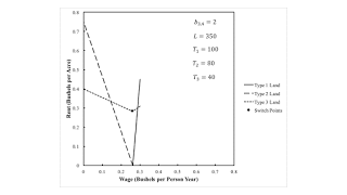
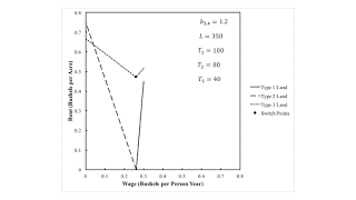
In the example, suppose two lands are fully cultivated, and one type of land is only partially cultivated. Figure 3 plots rents versus the wage for one value of the parameter b3, 4. For any given wage, one can sort land from the one with the highest rent, to a lower rent, to the type of land that pays no rent, given these assumptions. This is the order of rentability.
| Figure 3: Rents With a High Coefficient of Production for Type 3 Land |
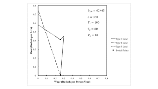
Figure 4 plots rents as a function of the wage for a slightly lower b3, 4. This perturbation leaves unchanged the location of wage curves in Figure 2. It does result in increased rents on type 3 lands though.
| Figure 4: A Fluke Coefficient of Production for Type 3 Land |
Figure 5 shows rents at an even lower b3, 4. I consider Figure 4 to be fluke case. Notice at the highest feasible wage in Figure 4, the rent per acre for type 1 and type 3 lands are equal. This fluke is associated with the disappearance of the range of the highes wages in which the order of rentability differs from the order of fertility.
| Figure 5: Rents With a Low Coefficient of Production for Type 3 Land |
Figure 1, at the top of this post, depicts a partition of a projection of the parameter space suggested by the above exploration. Employment is plotted against b3,4 the coefficient of projection for the land cultivated in the last process listed in Table 1. Each partition is a fluke case, in some sense. In each numbered region, the variation of the analysis of the choice of technique with distribution does not change qualitatively, while it does vary among regions. Table 3 specifies, for each region, which technique is cost-minimizing at a given wage and the range of employment. I consider the order of types of land by rent to be part of the analysis of the choice of technique. Table 3 specifies this order as well, along with its variation with the wage. A wage at which this order of rentability changes that is not a switch point in Figure 2 appears in regions 4, 6, and 7.
| Region | Wage | Technique | Summary |
| 1 | 0 < w < wmax | Mu | Type 3 land partially farmed. ρ1 = ρ2 = ρ3 = 0 |
| 2 | 0 < w < w* | Iota | Type 3 land fully farmed, type 2 land partially farmed. ρ1 = ρ2 = 0, ρ3 > 0 |
| w* < w < wmax | Theta | Type 3 land fully farmed, type 1 partially farmed. ρ1 = ρ2 = 0, ρ3 > 0 | |
| 3 | 0 < w < w* | Iota | Type 3 land fully farmed, type 2 land partially farmed. ρ1 = ρ2 = 0, ρ3 > 0 |
| w* < w < wmax | Gamma | Given wage, order of rentability is order of fertility. ρ2 = 0, ρ3 > ρ1 > 0 | |
| 4 | 0 < w < w* | Iota | Type 3 land fully farmed, type 2 land partially farmed. ρ1 = ρ2 = 0, ρ3 > 0 |
| w* < w < w1 | Gamma | Given wage, order of rentability is order of fertility. ρ2 = 0, ρ3 > ρ1 > 0 | |
| w1 < w < wmax | Gamma | Given wage, order of rentability is not order of fertility. ρ2 = 0, ρ1 > ρ3 > 0 | |
| 5 | 0 < w < w* | Beta | Given wage, order of rentability is order of fertility. ρ1 = 0, ρ3 > ρ2 > 0 |
| w* < w < wmax | Gamma | Given wage, order of rentability is order of fertility. ρ2 = 0, ρ3 > ρ1 > 0 | |
| 6 | 0 < w < w1 | Beta | Given wage, order of rentability is not order of fertility. ρ1 = 0, ρ2 > ρ3 > 0 |
| w1 < w < w* | Beta | Given wage, order of rentability is order of fertility. ρ1 = 0, ρ3 > ρ2 > 0 | |
| w* < w < wmax | Gamma | Given wage, order of rentability is order of fertility. ρ2 = 0, ρ3 > ρ1 > 0 | |
| 7 | 0 < w < w1 | Beta | Given wage, order of rentability is not order of fertility. ρ1 = 0, ρ2 > ρ3 > 0 |
| w1 < w < w* | Beta | Given wage, order of rentability is order of fertility. ρ1 = 0, ρ3 > ρ2 > 0 | |
| w* < w < w2 | Gamma | Given wage, order of rentability is order of fertility. ρ2 = 0, ρ3 > ρ1 > 0 | |
| w2 < w < wmax | Gamma | Given wage, order of rentability is not order of fertility. ρ2 = 0, ρ1 > ρ3 > 0 |
To illustrate the orders of fertility and rentability, consider a line segment running upwards through regions 1, 2, 4, and 7. Along such a line, employment increases. For a positive wage less than w*, the cost-minimizing technique is Mu, Iota, and Beta, depending on how much employment has expanded with the net final demand for corn. Thus, for a low wage, land is introduced into production, in order of declining fertility, as type 3, type 2, and type 1. In region 7, the order of lands from high rent to low, if the wage is between w1 and w*, is type 3, type 2, and type 1. If the wage is less than w1, the order from high rent to low, is type 2, type 3, and type 1. Whether or not the order of rentability matches the order of fertility can vary with distribution.
On the other hand, if the wage exceeds w*, the sequence of techniques associated with increasing final demand is Mu, Theta, and Gamma. That is, land, in order of decreasing fertility, is type 3, type 1, and type 2. The maximum wage decreases as less fertile land is taken under cultivation. The order of fertility itself depends on distribution. In this range of wages, region 7 also illustrates the dependence of the order of rentability on distribution.
Figures 3, 4, and 5 illustrate the partition around regions 7 and 6. A decrease of the coefficient b3,4 is associated with the loss of the possibility of a mismatch of the order of rentability and the order of fertility at high wages. A further decrease leads into region 5, where a mismatch in these orders is no longer possible at low rents. An even further decrease is associated with the least fertile lands being taken out of cultivation and the possibility of a larger economy.
Region 3 has an interesting property. The number of types of land that is farmed varies with distribution. For a low wage, workers in the corn industry are employed on types 2 and 3 land; type 1 land is left fallow and, along with type 2 land, pays no rent. For a high enough wage, types 1 and 3 land are fully farmed, and type 2 land is partially farmed and pays no rent. A landlord whose income is generated solely from ownership of type 1 land is better off if wages are high. Incidentally, here is a case in which the quantity demanded of a type of land is greater only when its price is higher.
6.0 ConclusionThis post illustrates that complications are introduced into my analysis of fluke switch points by considering models of land. In particular, I have located fluke parameters in which pertubations around these parameters result in the order of rentability varying from the order of fertility. This qualitative change is independent of switch points on intersecting wage curves. Obviously, this is one relatively simple example. I have a long ways to go in thinking about land.
References- J. E. Woods. 1990. The Production of Commodities: An Introduction to Sraffa. Atlantic Highlands: Humanities Press.
 Heterodox

