Table 1: A Common Structure Example1.0 Introduction This post presents partitions of (a part of) parameter space for two examples of models of prices of production with a choice of technique. The examples have a different structure and are parametrized differently. Yet, I want to argue, the partitions are the same, at some level of abstraction. 2.0 Thing 1 The first example is an instance of the Samuelson-Garegnani model. Table 1 presents the coefficients of production for this example. Each coefficient specifies the units of input needed to produce a unit output of the commodity for the given industry. Corn is the numeraire, and is not an input into any industry. It is non-basic in Sraffa's terminology. Three processes are available for producing corn, each distinguished by the
Topics:
Robert Vienneau considers the following as important: Example in Mathematical Economics, Sraffa Effects
This could be interesting, too:
Robert Vienneau writes Austrian Capital Theory And Triple-Switching In The Corn-Tractor Model
Robert Vienneau writes Double Fluke Cases For Triple-Switching In The Corn-Tractor Model
Robert Vienneau writes The Emergence of Triple Switching and the Rarity of Reswitching Explained
Robert Vienneau writes Recap For A Triple -Switching Example
| Table 1: A Common Structure Example |
This post presents partitions of (a part of) parameter space for two examples of models of prices of production with a choice of technique. The examples have a different structure and are parametrized differently. Yet, I want to argue, the partitions are the same, at some level of abstraction.
2.0 Thing 1The first example is an instance of the Samuelson-Garegnani model. Table 1 presents the coefficients of production for this example. Each coefficient specifies the units of input needed to produce a unit output of the commodity for the given industry. Corn is the numeraire, and is not an input into any industry. It is non-basic in Sraffa's terminology. Three processes are available for producing corn, each distinguished by the capital good used in that process. In a technique, the process that produces that capital good and the given corn-producing process are operated. The techniques are labeled Alpha, Beta, and Gamma, depending on the corn-producing process. The example is fully specified by assigning values to a2,2 and a3,3.
| Input | Industry | |||||
| Iron | Copper | Uranium | Corn | |||
| Alpha | Beta | Gamma | ||||
| Labor | 1 | 17328/8281 | 1 | 1 | 361/91 | 3.63505 |
| Iron | 1/2 | 0 | 0 | 3 | 0 | 0 |
| Copper | 0 | a2,2 | 0 | 0 | 1 | 0 |
| Uranium | 0 | 0 | a3,3 | 0 | 0 | 1.95561 |
| Corn | 0 | 0 | 0 | 0 | 0 | 0 |
Given the technique (with the parameters assigned numberical values) and, say, a feasible rate of profits, one can solve for the real wage and prices of production. At each feasible rate of profits, the choice of technique is determined by cost. It is the cost-minimizing one. In general, the choice of technique varies with the rate of profits. One could also take the wage as given, and find the rate of profits as a function of the wage.
To go on, I draw upon my publications. I call a switch point in which two wage curves are tangent at that point a reswitching pattern (of switch points). A three-technique pattern (of switch points) is a switch point in which three wage curves intersect. Both of these patterns exist in this example.
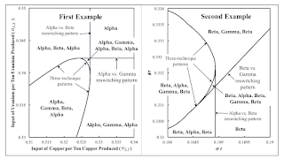
The left panel in Figure 1 above partitions a portion of the parameter space for this model. I label each region by the cost-minimizing techniques along the wage frontier, in the order of an increasing rate of profits. The partitions are labeled by the corresponding pattern of switch points. This case illustrates how a perturbation of coefficients of production can lead to the emergence of the reswitching of techniques.
3.0 Thing 2In the second example, two commodities are produced, and they both are basic commodities in all three techniques. Table 2 presents the coefficients of production for this example. I have introduced technological change in this model The coefficients of production for producing corn with the Beta and Gamma processes decrease exponentially. They decrease at different rates for the two processes, but all coeficients for a process descrease at the same rate.
| Input | Industry | |||
| Iron | Corn | |||
| Alpha | Beta | Gamma | ||
| Labor | 1 | 5191/5770 | (305/494) e(3/20) - σt | (19/20) e(3/10) - φt |
| Iron | 9/20 | 1/40 | (3/1976) e(3/20) - σt | (1/40) e(3/10) - φt |
| Corn | 2 | 1/10 | (229/494) e(3/20) - σt | (1/10) e(3/10) - φt |
Given the coefficients at a particular time, one can find prices of production and the cost-minimizing technique. Here, too, the analysis of the choice of technique can be performed by constructing the wage frontier. The model is parametrized by (σ t) and (φ t). The right panel in Figure 1 shows a portion of this parameter space for this model.
4.0 ConclusionI want to say that the two panels in Figure 1 depict the same structure. The labeling of techniques is different, and one panel requires the other be rotated and stretched, as is typical of topological structures. In both cases, the loci for two reswitching patterns intersects. At that intersection, one wage curve on the wage frontier is tangent to two other wage curves, each at a separate switch point. Each locus for the reswitching patterns terminates at a point of tangency for a locus of three-technique patterns. And a three-technique pattern forms an arc connecting those two points of tangency.
Other common structures can be found in the parameter spaces of models of prices of production with the choice of technique.l
 Heterodox

