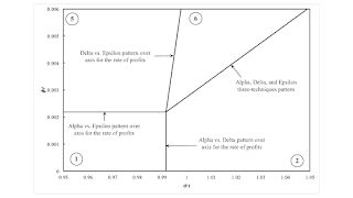
Figure 1: Three Patterns Across the r Axis and One Three-Technique Pattern This post begins a perturbation analysis of an example of intensive rent from D'Agata. I have previously claimed that certain structures in parameter space are universal in some sense. Table 1 presents the available technology. Corn is grown on homogeneous land, and three processes are available for producing corn. One hundred acres of land are available, leading to the possibility of two processes being operated side-by-side with positive rent. Processes III and IV undergo technical progress through time. Table 2 shows the processes operated in each of the six techniques available. Table 1: The Coefficients of Production InputIndustries and ProcessesIronSteelCornIIIIIIIVVLabor111(11/5) e(5/4) - σte(1/20) -
Topics:
Robert Vienneau considers the following as important: Example in Mathematical Economics, Joint Production
This could be interesting, too:
Robert Vienneau writes Austrian Capital Theory And Triple-Switching In The Corn-Tractor Model
Robert Vienneau writes Double Fluke Cases For Triple-Switching In The Corn-Tractor Model
Robert Vienneau writes The Emergence of Triple Switching and the Rarity of Reswitching Explained
Robert Vienneau writes Recap For A Triple -Switching Example
| Figure 1: Three Patterns Across the r Axis and One Three-Technique Pattern |
This post begins a perturbation analysis of an example of intensive rent from D'Agata. I have previously claimed that certain structures in parameter space are universal in some sense.
Table 1 presents the available technology. Corn is grown on homogeneous land, and three processes are available for producing corn. One hundred acres of land are available, leading to the possibility of two processes being operated side-by-side with positive rent. Processes III and IV undergo technical progress through time. Table 2 shows the processes operated in each of the six techniques available.
| Input | Industries and Processes | ||||
| Iron | Steel | Corn | |||
| I | II | III | IV | V | |
| Labor | 1 | 1 | 1 | (11/5) e(5/4) - σt | e(1/20) - φt |
| Land | 0 | 0 | 1 | e(5/4) - σt | e(1/20) - φt |
| Iron | 0 | 0 | 1/10 | (1/10) e(5/4) - σt | (1/10) e(1/20) - φt |
| Steel | 0 | 0 | 2/5 | (1/10) e(5/4) - σt | (1/10) e(1/20) - φt |
| Corn | 1/10 | 3/5 | 1/10 | (3/10) e(5/4) - σt | (2/5) e(1/20) - φt |
| Technique | Process |
| Alpha | I, II, III |
| Beta | I, II, IV |
| Gamma | I, II, V |
| Delta | I, II, III, IV |
| Epsilon | I, II, III, V |
| Zea | I, II, IV, V |
Requirements for use are 90 tons iron, 60 tons steel, and 19 bushels corn. In this parameter range, Alpha, Delta, and Epsilon can meet requirements for use. That is, one can find levels of operation of the processes comprising these techniques such that the net output of the economy is the previously specified vector and no more than 100 acres of land are farmed. Beta, Gamma, and Zeta are infeasible.
Figure 1, at the top of this post, illustrates a part of the parameter space formed by (σ t) and (φ t). Patterns of fluke switch points partition the parameter space into regions in which the wage frontier does not qualitatively vary within each region. (From the numbering, you may correctly guess other patterns of fluke switch points form other partitions off the edges of the graph.)
| Region | Range | Technique | Notes |
| 1 | 0 ≤ r ≤ Rα | Alpha | No rent. |
| 2 | 0 ≤ r ≤ r1 | Alpha | Non-unique cost-minimizing technique. Wage curve for Delta slopes up on frontier. |
| r1 ≤ r ≤ r2 | Alpha, Delta | ||
| 5 | 0 ≤ r ≤ r1 | Alpha | Positive rent for some range of the rate of profits. |
| r1 ≤ r ≤ Rε | Epsilon | ||
| 6 | 0 ≤ r ≤ r1 | Alpha | Non-unique cost-minimizing technique. Wage curve for Delta slopes up on frontier. |
| r1 ≤ r ≤ r2 | Epsilon | ||
| r2 ≤ r ≤ r3 | Delta, Epsilon |
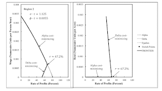
| Figure 2: Wage Frontier and Rent in Region 2 |
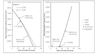
| Figure 3: Wage Frontier and Rent in Region 5 |
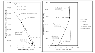
| Figure 4: Wage Frontier and Rent in Region 6 |
One can summarize, as in Table 3, which switch points and wage curves appear on the frontier in each region. In region 1, the Alpha technique is cost-minimizing for all rates of profits. Land is in excess supply, and no rent is formed. Technical progress is modeled by a movement to the east, north, or northeast in Figure 1. Technical progress here eventually results in land being scarce, at least for some range of the rate of profits, and landlords receiving a rent. Figures 2, 3, and 4 show the wage frontiers and rent per acre, as a correspondence with the rate of profits, for regions 2, 5, and 6.
Some phenomena arise in regions 2 and 6 that are not possible in models with circulating capital alone. As I understand it, these phenomena are also not possible in pure fixed capital models and in models of extensive rent. I am referring specifically to upward-sloping wage curves on the frontier and a non-unique cost-minimizing technique for some rates of profits.
I like that despite these oddities, the illustrated partition of the selected part of the parameter space is qualitatively similar to partitions for parts of parameter spaces for circulating capital models. Maybe I am exploring something fundamental underlying the analysis of the choice of technique.
 Heterodox


