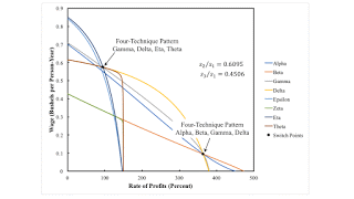
Figure 1: Wage Curves for the Example1.0 Introduction The Cambridge Capital Controversy (CCC) applies to models both of competitive industries and of non-competitive industries. Around a switch point exhibiting capital-reversing, a higher wage is associated with greater employment per unit of net output produced. It is not merely a question of what technology is available. It is also a matter of the power of firms among industries to extract value from their workers, their upstream suppliers, and their downstream buyers. And of the countervailing power to resist such exercise of power. Can you cite literature in Industrial Organization (IO) that explicitly recognizes the logical consequences of the CCC for IO? This post presents an example of a fluke switch point, or rather two fluke
Topics:
Robert Vienneau considers the following as important: Full Cost Prices, Sraffa Effects
This could be interesting, too:
Robert Vienneau writes Three Examples For The Cambridge Capital Controversy
Robert Vienneau writes Variations In Switch Points With Markups In The ‘Corn’ Industry
Robert Vienneau writes Reswitching Pattern In Corn-Tractor Model
Robert Vienneau writes Wages, Employment Not Determined By Supply And Demand
| Figure 1: Wage Curves for the Example |
The Cambridge Capital Controversy (CCC) applies to models both of competitive industries and of non-competitive industries. Around a switch point exhibiting capital-reversing, a higher wage is associated with greater employment per unit of net output produced. It is not merely a question of what technology is available. It is also a matter of the power of firms among industries to extract value from their workers, their upstream suppliers, and their downstream buyers. And of the countervailing power to resist such exercise of power. Can you cite literature in Industrial Organization (IO) that explicitly recognizes the logical consequences of the CCC for IO?
This post presents an example of a fluke switch point, or rather two fluke switch points, in a global pattern. It is a case in which capital-reversing just begin to arise.
2.0 TechnologyI have used an example with this structure before. This economy produces a single consumption good, called corn. Corn is also a capital good, that is, a produced commodity used in the production of other commodities. In fact, iron, steel, and corn are capital goods in this example. So three industries exist. One produces iron, another produces steel, and the last produces corn. Two processes exist in each industry for producing the output of that industry. Each process exhibits Constant Returns to Scale (CRS) and is characterized by coefficients of production. Coefficients of production (Table 1) specify the physical quantities of inputs required to produce a unit output in the specified industry. All processes require a year to complete, and the inputs of iron, steel, and corn are all consumed over the year in providing their services so as to yield output at the end of the year.
| Input | Iron Industry | Steel Industry | Corn Industry | |||
| a | b | c | d | e | f | |
| Labor | 1/3 | 1/10 | 5/2 | 7/20 | 1 | 3/2 |
| Iron | 1/6 | 2/5 | 1/200 | 1/100 | 1 | 0 |
| Steel | 1/200 | 1/400 | 1/4 | 3/10 | 0 | 1/4 |
| Corn | 1/300 | 1/300 | 1/300 | 0 | 0 | 0 |
A technique consists of a process in each industry. Table 2 specifies the eight techniques that can be formed from the processes specified by the technology. If you work through this example, you will find that to produce a net output of one bushel corn, inputs of iron, steel, and corn all need to be produced to reproduce the capital goods used up in producing that bushel.
| Technique | Processes |
| Alpha | a, c, e |
| Beta | a, c, f |
| Gamma | a, d, e |
| Delta | a, d, f |
| Epsilon | b, c, e |
| Zeta | b, c, f |
| Eta | b, d, e |
| Theta | b, d, f |
I consider prices of production in which:
- Labor is advanced and is paid out of the surplus product at the end of the year.
- Firms in differenct industries are able to enforce barriers to entry, with stable ratios of profits among industries.
- A bushel of corn is the numeraire.
Let s1r be the rate of profits in the iron industry, s2r be the rate of profits in the steel industry, and s1r be the rate of profits in the corn industry. I consider the case with s1 set to unity, and the ratio of the other two markups to this as noted in the figures in this post. Maybe I should go back to calling r the scale factor for the rate of profits.
Under these assumptions, a system of three equations can be set out for the three techniques. The variables in these equations are the rate of profits r, the wage, the price of iron, and the price of steel. They can be solved with one degree of freedom remaining open. Figure 1, at the top of this post, shows the wage curves for each technique. The wage curves for the Zeta and Theta techniques, at least, are more curved than is typically found in the empirical literature.
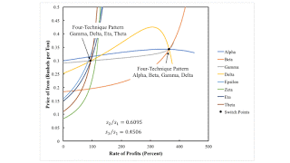
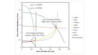
One can also find the price of iron and steel, as shown in Figures 2 and 3 below. At a switch point, the wage and prices are the same for all techniques on the frontier.
| Figure 2: The Price of Iron in the Example |
| Figure 3: The Price of Steel in the Example |
At the first switch point, managers of firms in the iron and corn industry do not care which of the two processes in their industry they operate. Contrawise, at the other switch point, managers of firms in steel industry and the corn industry do not care.
4.0 ConclusionThis combination of fluke switch points is an intersection of two one-dimensional manifolds in the two-dimensional parameter space formed by the relative markups, s2/s1 and s3/s1. Each manifold characterizes one of the two four-technique fluke switch points. I do not think I have yet constructed an example of manifolds partitioning such a two-dimensional space of relative markups.
 Heterodox


