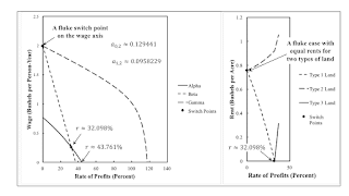
Figure 1: Wage Curves and Rent for an Example of Extensive Rent This is basically an introduction to a draft research article. Maybe I have difficulty in justifying paying attention to the type of fluke points I haqve been exploring and in formally defining why they are flukes. In this post, I present a partition of a parameter space associated with an example of extensive rent. It is probably too complicated to replace this example. Anyways, I have constructed a new fluke case. Here a switch point associated with a variation in the order of fertility is also associated with a variation in the order of rentability. I suppose one can read David Ricardo as mistakenly thinking this was the general case. The analysis of the choice of technique in models of extensive rent can be based on
Topics:
Robert Vienneau considers the following as important: Example in Mathematical Economics, Joint Production, Sraffa Effects
This could be interesting, too:
Robert Vienneau writes Austrian Capital Theory And Triple-Switching In The Corn-Tractor Model
Robert Vienneau writes Double Fluke Cases For Triple-Switching In The Corn-Tractor Model
Robert Vienneau writes The Emergence of Triple Switching and the Rarity of Reswitching Explained
Robert Vienneau writes Recap For A Triple -Switching Example
| Figure 1: Wage Curves and Rent for an Example of Extensive Rent |
This is basically an introduction to a draft research article. Maybe I have difficulty in justifying paying attention to the type of fluke points I haqve been exploring and in formally defining why they are flukes.
In this post, I present a partition of a parameter space associated with an example of extensive rent. It is probably too complicated to replace this example. Anyways, I have constructed a new fluke case. Here a switch point associated with a variation in the order of fertility is also associated with a variation in the order of rentability. I suppose one can read David Ricardo as mistakenly thinking this was the general case.
The analysis of the choice of technique in models of extensive rent can be based on the construction of wage curves, even though the outer envelope does not represent the cost-minimizing technique. The orders of fertility and rentability are emphasized here. The order of fertility is defined for specified techniques, in which a single quality of land is used in each technique and that land pays no rent. At a given rate of profits, the qualities of land are ordered by wages, with the most fertile land paying the highest wage. The order of rentability specifies the sequence of different qualities of lands from high rent per acre to low rent per acre. Both orders may vary with the wage or the rate of profits. Table 1 presents coefficients of production for an example.
| Input | Iron Industry | Corn Industry | ||
| I | II | III | IV | |
| Labor | 1 | a0,2 | 91/250 | 67/100 |
| Type 1 Land | 0 | 49/100 | 0 | 0 |
| Type 2 Land | 0 | 0 | 59/100 | 0 |
| Type 3 Land | 0 | 0 | 0 | 9/20 |
| Iron | 9/20 | a1,2 | 9/10000 | 67/1000 |
| Corn | 2 | 6/125 | 27/100 | 3/20 |
How much corn can be produced is constrained by the available quantities of each type of land. Endowments of land and requirements for use must be among the givens to analyze the choice of technique in this example. Suppose one hundred acres of each type of land are available, and net output is such that all three types of land must be farmed. One type will be only partially farmed. The iron-producing process must be operated in each of the three economically viable techniques. Table 2 describes which type of lands are fully cultivated and which type of land is left partially fallow in each of the Alpha, Beta, and Gamma techniques.
| Technique | Land | ||
| Type 1 | Type 2 | Type 3 | |
| Alpha | Fully farmed | Fully farmed | Partially farmed |
| Beta | Partially farmed | Fully farmed | Fully farmed |
| Gamma | Fully farmed | Partially farmed | Fully farmed |
For a given technique, the rent on a type of land only partially farmed is zero since it is not scarce. The wage curves in the left pane in Figure 1 are constructed, for each technique, from the price equations provided by the iron-producing process and the corn-producing process for the land that pays no rent. The choice of technique depends on both income distribution and requirements for use (Quadrio-Curzio 1980). Suppose the rate of profits is taken as given. Then the r–order of efficiency or fertility is the order of the wage curves downwards, until requirements for use are satisfied. Since all three types of land must be somewhat cultivated in the example, the wage frontier is the inner envelope of the wage curves. For the illustrated parameters, Alpha is cost-minimizing, and the order of fertility between the switch points Type 2, Type 1, and Type 3 lands. At the switch point on the wage axis, Type 1 and Type 2 lands are equally fertile. For rates of profits exceeding that at the second switch point, the order of fertility is Type 2, Type 3, and Type 1 lands.
One can calculate the cost of capital goods at the given rate of profits and the cost of labor inputs for corn-producing processes on each land that pays a rent. Since coefficients of production are specified per bushel corn produced, the revenues from each of these processes, at a unit level, are the same as the process operated on the least fertile land, which pays no rent. Rent is the difference between revenues and non-land costs on scarce lands. Rent per acre is plotted in the right pane for Figure 1. The order of rentability is the order of lands by rent per acre. The order of rentability is the same as the order of fertility for the given parameters.
The example in Figure 1 is a fluke case at a rate of profits of zero is a fluke case three times over. A switch point on the outer frontier lies on the wage axis. The rent per acre for Type 1 and Type 2 lands is the same at a rate of profits of zero. And the order of efficiency and the order of rentability both change, in some sense, at a rate of profits of zero.
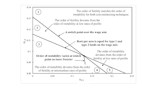
| Figure 2: A Portion of the Parameter Space |
To the northeast in Figure 2 (Region 1), the switch point at a rate of profits of zero has disappeared over the wage axis. The order of fertility matches the order of rentability, even with the variation in the choice of technique with distribution. To the northwest (Region 2), this switch point appears at a positive rate of profits, and the order of fertility varies with the rate of profits where the Alpha technique is cost-minimizing. The point of intersection on the right-hand pane in Figure 1 still occurs at a rate of profits of zero. Towards the southwest (Region 3), this intersection occurs at a positive rate of profits, but still at a smaller rate of profits than the switch point for which the order of fertility varies for the Alpha technique. The order of fertility and the order of rentability are the same at a rate of profits of zero, but reversed from what they are in Region 1. Region 3 and Region 4 differ in that the switch point for which the order of fertility varies for the Alpha technique occurs at a rate of profits less than the rate of profits at which the rent per acre for Type 1 and Type 2 lands are equal. Finally, the range of profits for which the rate of fertility differs, for the Alpha tecnique, from what it is in Region 1 has vanished. Table 3 summarizes this discussion.
| Region | Range | Land Partially Farmed | Order of Fertility | Order of Rentability |
| 1 | 0 ≤ r ≤ r1 | Type 3 | Type 2 > Type 1 | Type 2 > Type 1 |
| r1 ≤ r ≤ Rβ | Type 1 | Type 2 > Type 3 | Type 2 > Type 3 | |
| 2 | 0 ≤ r ≤ r1 | Type 3 | Type 1 > Type 2 | Type 2 > Type 1 |
| r1 ≤ r ≤ r2 | Type 2 > Type 1 | |||
| r2 ≤ r ≤ Rβ | Type 1 | Type 2 > Type 3 | Type 2 > Type 3 | |
| 3 | 0 ≤ r ≤ r1 | Type 3 | Type 1 > Type 2 | Type 1 > Type 2 |
| r1 ≤ r ≤ r2 | Type 2 > Type 1 | |||
| r2 ≤ r ≤ r3 | Type 2 > Type 1 | |||
| r3 ≤ r ≤ Rβ | Type 1 | Type 2 > Type 3 | Type 2 > Type 3 | |
| 4 | 0 ≤ r ≤ r1 | Type 3 | Type 1 > Type 2 | Type 1 > Type 2 |
| r1 ≤ r ≤ r2 | Type 2 > Type 1 | |||
| r2 ≤ r ≤ r3 | Type 2 > Type 1 | |||
| r3 ≤ r ≤ Rβ | Type 1 | Type 2 > Type 3 | Type 2 > Type 3 | |
| 5 | 0 ≤ r ≤ r1 | Type 3 | Type 2 > Type 1 | Type 1 > Type 2 |
| r1 ≤ r ≤ r2 | Type 2 > Type 1 | |||
| r2 ≤ r ≤ Rβ | Type 1 | Type 2 > Type 3 | Type 2 > Type 3 |
The correct analysis of extensive rent does not conform to reasoning based on supply and demand. If you disagree, can you tell a supply and demand story for this example? I find it difficult to directly confront these two modes of reasoning, one correct and one known, for decades, to be confused. I also want to say that partitioning parameter spaces with fluke switch points can illuminate the impact of technical change on income dynamics. A movement from the northeast to the southwest in Figure 2 is an improvement in technology. Such an improvement has an impact on how landlords view struggles between capitalists and workers over the rate of profits and wages. But I am still putting aside the difficult question of the supposed tendency of market prices to approach prices of production.
 Heterodox


