Figure 1: Order of Rentability Varying with Relative Markups1.0 Introduction Ownership is not productive, as Joan Robinson informs us. But, at least under competitive conditions one might hope, more productive assets earn their owners more than less productive assets. And this applies to scarce skills as well. But none of this is necessarily true, either. This article presents a numerical example in which, among scarce lands, rent per acre is higher on more fertile land only when capitalists in agriculture have more market power than industrial capitalists. Only the unenlightened would assess one’s worth by how much income they are able to obtain from what they own. A less efficient scarce asset can receive a higher rent. The proof of this statement is provided by a model of the
Topics:
Robert Vienneau considers the following as important: Full Cost Prices, Joint Production, rent
This could be interesting, too:
Robert Vienneau writes Variations In An Analysis Of Intensive Rent With One Type Of Land (Part 2/2)
Robert Vienneau writes Variations In An Analysis Of Intensive Rent With One Type Of Land (Part 1/2)
Robert Vienneau writes Intensive Rent With Two Types Of Land
Robert Vienneau writes Intensive Rent And The Order Of Rentability
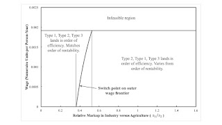
| Figure 1: Order of Rentability Varying with Relative Markups |
Ownership is not productive, as Joan Robinson informs us. But, at least under competitive conditions one might hope, more productive assets earn their owners more than less productive assets. And this applies to scarce skills as well. But none of this is necessarily true, either. This article presents a numerical example in which, among scarce lands, rent per acre is higher on more fertile land only when capitalists in agriculture have more market power than industrial capitalists. Only the unenlightened would assess one’s worth by how much income they are able to obtain from what they own.
A less efficient scarce asset can receive a higher rent. The proof of this statement is provided by a model of the production of commodities by means of commodities with land. No imperfections, such as externalities, asymmetric information, transactions costs, and so on exist in the model. More fertile lands are more efficient. The order of efficiency of types of land is the order in which they are introduced into cultivation as requirements for use expand, given the wage. Lands can also be ordered by rent per acre, with non-scarce lands being fallow or only partially cultivated. Lands that are not scarce receive a rent of zero.
The existence of market power is shown by markup pricing. When markups in agriculture and industry are equal and the economy is competitive, here the order of efficiency is opposite from the order of rentability for scarce lands. The order of efficiency varies when agriculture has sufficient market power. Only when agriculture has sufficient market power does the order of efficiency match the order of rentability.
As far as I know, this is the first explicit presentation of a model of the prices of production with extensive rent. Kurz & Salvadori (1995), Quadrio-Curzio (1980), and Schefold (1989) treat rent, including extensive rent. D'Agata (2018), Steedman (1981), Vienneau (2023), and Zambelli (2018) modify Sraffa's equations for prices of production to include markup pricing.
2.0 TechnologyTable 1 presents the technology for the example. The second column shows the inputs of labor, iron, and corn needed to produce a ton of iron. The remaining three columns to the right are the coefficients of production for processes to produce corn. A unit level of operation of a process in agriculture produces a bushel corn and requires an input of one of three types of land, as shown. Constant returns to scale prevail, although the level of operation of the processes producing corn is limited by the available acreage.
| Input | Industry | |||
| Iron | Corn | |||
| I | II | III | IV | |
| Labor | a0,1 = 1 | a0,2 = 11/25 | a0,3 = 91/250 | a0,4 = 67/100 |
| Type I Land | 0 | c1,2 = 49/100 | 0 | 0 |
| Type II Land | 0 | 0 | c2,3 = 59/100 | 0 |
| Type III Land | 0 | 0 | 0 | c3,4 = 9/20 |
| Iron | a1,1 = 9/20 | a1,2 = 1/100 | a1,3 = 9/10000 | a1,4 = 67/1000 |
| Corn | a2,1 = 2 | a2,2 = 6/125 | a2,3 = 27/100 | a2,4 = 3/20 |
The given data also include the land available and the requirements for use. These are such that all three type of land must be at least partially farmed. Specifically, 100 acres of each type of land exist, and net output consists of 400 bushels corn. Four hundred bushels of corn is taken as the numeriare.
Three techniques, Alpha, Beta, and Gamma, can feasibly satisfy requirements for use. In all three techniques, all four processes are operated. One of the types of land is not fully cultivated in each technique. Table 2 displays which type of land is only partially cultivated in each technique. The choice of technique is based on cost-minimization or profit maximization.
| Technique | Land | ||
| Type 1 | Type 2 | Type 3 | |
| Alpha | Partially farmed | Fully farmed | Fully farmed |
| Beta | Fully farmed | Partially farmed | Fully farmed |
| Gamma | Fully farmed | Fully farmed | Partially farmed |
| Variable | Definition |
| s1 | Relative markup in industry. |
| s2 | Relative markup in agriculture. |
| r | Scale factor for the rate of profits. |
| ρ1 | The rent on Type 1 land. |
| ρ2 | The rent on Type 2 land. |
| ρ3 | The rent on Type 3 land. |
| w | The wage. |
Prices of production are specified by a system of equations with one degree of freedom. Table 3 defines the variables in these equations. Prices of production satisfy the following system of equations:
(p1a1,1 + p2a2,1)(1 + s1r) + w a0,1 = p1
(p1a1,2 + p2a2,2)(1 + s2r) + ρ1c1,2 + w a0,2 = p2
(p1a1,3 + p2a2,3)(1 + s2r) + ρ2c2,3 + w a0,3 = p2
(p1a1,4 + p2a2,4)(1 + s2r) + ρ3c3,4 + w a0,4 = p2
I am assuming that wages and rents are paid out of the surplus at the end of the period of production. The relative market power of industry over industry, or vice versa, is expressed by the ratio s1/s2. When this ratio is unity, the equations characterize a competitive capitalist economy. The following equation specifies that the rent on at least one type of land is zero:
ρ1 ρ2 ρ3 = 0
Finally, let the price of the commodity basket consisting of the numeraire be unity:
400 p2 = 1
This completes the exposition of the equations specifying prices of production.
The above system of equations can be solved given the technique, the markups for industry and agriculture, and the wage. For a given technique, one of the equations for agriculture processes is picked out as being operated at a positive level with a rent of zero. The equation for the industrial process and for this process is a system of equations in four variables: the scale factor for the rates of profit, the wage, the price of iron, and the price of corn. (I am taking the scale factors as given.) The numeraire in this case fixes the price of corn. It is convenient to take the scale factor as given to obtain the wage and the price of iron as functions of the scale factor of the rate of profits. Each of the other equations for the agricultural processes can then be used to obtain rent per acres on scarce lands as functions of either the scale factor or the wage.
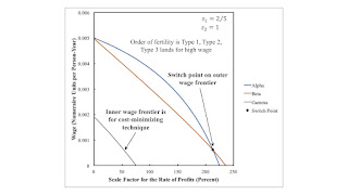
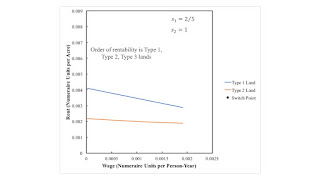
4.0 The Choice of TechniqueFigures 2 and 3 illustrate prices of production for specific markups, in which agriculture has some market power, as compared to industry. Figure 2 displays the wage as a function of the scale factor for the rate of profits. It is a general property in a model of extensive rent that these wage curves slope down to the right. Thus, one can also view this graph as showing the scale factor as a function of the wage, given markups and the technique. Figure 3 graphs rent per acre, for the scarce lands when the Gamma technique is adopted, as a function of the wage, with markups given.
| Figure 2: Wage Curves with Agriculture Having Market Power |
| Figure 3: Rent Curves with Agriculture Having Market Power |
At a given rate wage, order the wage curves on the left pane in Figure 2 from the right to the left. This is the order of fertility, also known as the order of efficiency. A specific type of land with a rent of zero is associated with each technique. If requirements for use could be satisfied by farming just one type of land, type 1 land would be the only land farmed at a feasible wage above the switch point, given the markups. That is the economically most efficient process for growing corn maximizes the rate of profits, given the wage. Economic efficiency, generally, varies from technical efficiency and varies with distribution.
But suppose two types of land must be farmed to satisfy requirements for use. Then, given high wages, the land associated with the Beta technique would be brought under cultivation. Type 2 land would be farmed and obtain no rent.
Under the assumption that all three types of land must be farmed to satisfy requirements for use, the Gamma technique is adopted for any feasible wage. The maximum feasible wage is lower than when two types of lands can satisfy requirements for use. The order of efficiency for high wages is Type 1, Type 2, and Type 3 lands for high wage. It is Type 2, Type 1, and Type 3 for low wages.
Since only the Gamma technique is cost minimizing in the illustrated case, only the rent curves for Gamma are graphed in Figure 3. The order of rentability, from high rent per acre down, is Type 1, Type 2, and Type 3 lands. The order of efficiency does not match the order of rentability for low wages.
5.0 Economic Efficiency Varying with Relative Markups and the WageHow does the above analysis vary with relative markups? Consider Figure 1 at the top of this post. For this numerical example, Gamma is always cost-minimizing for all feasible wages, whatever relative markups in industry and agriculture. Thus, the maximum feasible wage is a horizontal line at the top of the graph. The rent curves never intersect with variation in relative markups. The order of rentability does not change. The order of efficiency does change, however. Figure 1 plots the wage at which the Alpha and Beta wage curves intersect.
The thin vertical lines in Figure 1 are fluke cases. The left-most case arises when the Alpha and Beta wage curves intersect at a wage of zero. The rightmost case occurs when these wage curves intersect at the maximum feasible wage for Gamma.
Anyways the order of efficiency does not vary with the wage for sufficiently high market power for agriculture. On the left in Figure 1, the order of efficiency matches the order of rentability for all feasible wages. On the right, including the competitive case, the order of efficiency differs from the order of rentability. The variation of the order of efficiency with the wage is an intermediate case.
This example does not illustrate some of the possibilities of the theory of extensive rent. In general, the cost-minimizing technique varies with the wage. The order of efficiency varies with the technique. As illustrated, the order of efficiency can vary with the wage, even in a range of the wage in which a single technique is cost-minimizing. The order of rentability also varies with the technique, including which lands are scarce. And the order of rentability can vary in a range of the wage in which a single technique is cost-minimizing. That is the rent curves for a single technique may intersect.
6.0 ConclusionThis article builds on Ricardian theory done right. Karl Marx, in the third volume of Capital, does not go deep enough. He does, however, have some insights on the dynamics of rent. He is correct in his mocking of the trinty formula. Whether you want to say that the variation of the dependence of rent on wages on relative markups is an illustration of his concept of absolute rent is a matter of taste, I guess.
Anyways, I have proven my original claim. An asset, for example, a type of land, may obtain a larger rent than another asset even though processes that use the latter asset are more economically efficient. It is only when agriculture has sufficient market power in the example that, given the wage, the ordering of lands by economic efficiency matches the ordering of lands by rent.
References- Deepankar Basu, 2022. A Reformulated Version of Marx’s Theory of Ground-Rent Shows that there Cannot be any Absolute Rent. Review of Radical Political Economy 54(4)
- D'Agata, A. 2018. Freeing Long-Period Prices from the Uniform Profit Rate Hypothesis: A General Model of Long-Period Positions. Metroeconomica 69 (4): 847–861.
- Kurz, H. D. and N. Salvadori (1995) Theory of Production: A Long-Period Analysis, Cambridge: Cambridge University Press.
- Quadrio-Curzio, A. (1980) Rent, income distribution, and orders of efficiency and rentability, in Pasinetti, L. L. (ed.) Essays on the Theory of Joint Production, New York: Columbia University Press.
- Schefold, B. (1989) Mr. Sraffa on Joint Production and other Essays, London: Unwin-Hyman.
- Steedman, I. 1981. Marx After Sraffa. London: Verso.
- Vienneau, R. L. (2023) Characteristics of labor markets varying with perturbations of relative markups, Review of Political Economy To appear.
- Zambelli, S. 2018. Production of Commodities by Means of Commodities and Non-Uniform Rates of Profits. Metroeconomica 69 (4): 791–819.
 Heterodox


