Figure 1: Wage Curves and Rent for an Example of Extensive Rent I more-or-less have a draft research article in five posts: post 1 post 2 post 3 post 4 post 5. I suggest that the current post can replace the fourth post. It is a variant on on this post. The analysis of the choice of technique in models of extensive rent can be based on the construction of wage curves, even though the outer envelope does not represent the cost-minimizing technique. The orders of fertility and rentability are emphasized here. The order of fertility is defined for specified techniques, in which specified qualities of land are farmed, with one quality only partially farmed. Being in excess supply, the partially farmed land pays no rent. At a given rate of profits, the qualities of land are ordered by wages,
Topics:
Robert Vienneau considers the following as important: Example in Mathematical Economics, rent, Sraffa Effects
This could be interesting, too:
Robert Vienneau writes Austrian Capital Theory And Triple-Switching In The Corn-Tractor Model
Robert Vienneau writes Double Fluke Cases For Triple-Switching In The Corn-Tractor Model
Robert Vienneau writes The Emergence of Triple Switching and the Rarity of Reswitching Explained
Robert Vienneau writes Recap For A Triple -Switching Example
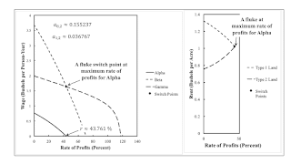
| Figure 1: Wage Curves and Rent for an Example of Extensive Rent |
I more-or-less have a draft research article in five posts: post 1 post 2 post 3 post 4 post 5. I suggest that the current post can replace the fourth post. It is a variant on on this post.
The analysis of the choice of technique in models of extensive rent can be based on the construction of wage curves, even though the outer envelope does not represent the cost-minimizing technique. The orders of fertility and rentability are emphasized here. The order of fertility is defined for specified techniques, in which specified qualities of land are farmed, with one quality only partially farmed. Being in excess supply, the partially farmed land pays no rent. At a given rate of profits, the qualities of land are ordered by wages, with the most fertile land paying the highest wage. The order of rentability specifies the sequence of different qualities of lands from high rent per acre to low rent per acre. Both orders may vary with the wage or the rate of profits. Table 1 presents coefficients of production for an example.
| Input | Iron Industry | Corn Industry | ||
| I | II | III | IV | |
| Labor | 1 | a0,2 | 91/250 | 67/100 |
| Type 1 Land | 0 | 49/100 | 0 | 0 |
| Type 2 Land | 0 | 0 | 59/100 | 0 |
| Type 3 Land | 0 | 0 | 0 | 9/20 |
| Iron | 9/20 | a1,2 | 9/10000 | 67/1000 |
| Corn | 2 | 6/125 | 27/100 | 3/20 |
The quantity of corn that can be produced is constrained by the available quantities of each type of land. Endowments of land and requirements for use must be among the givens to analyze the choice of technique in this example. Suppose one hundred acres of each type of land are available, and net output is somewhere between 302 and 424 bushels of corn. Then all three types of land must be farmed with the parameters specified in Figure 1. One type will be only partially farmed. The iron-producing process must be operated in each of the three economically viable techniques. Table 2 describes which type of lands are fully cultivated and which type of land is left partially fallow in each of the Alpha, Beta, and Gamma techniques.
| Technique | Land | ||
| Type 1 | Type 2 | Type 3 | |
| Alpha | Fully farmed | Fully farmed | Partially farmed |
| Beta | Partially farmed | Fully farmed | Fully farmed |
| Gamma | Fully farmed | Partially farmed | Fully farmed |
For a given technique, the rent on a type of land only partially farmed is zero since it is not scarce. The wage curves in the left pane in Figure 1 are constructed, for each technique, from the price equations provided by the iron-producing process and the corn-producing process for the land that pays no rent. The choice of technique depends on both income distribution and requirements for use (Quadrio-Curzio 1980). Suppose the rate of profits is taken as given. Then the r–order of efficiency or fertility is the order of the wage curves downwards, until requirements for use are satisfied. Since all three types of land must be somewhat cultivated in the example, the wage frontier is the inner envelope of the wage curves. For the illustrated parameters, Alpha is cost-minimizing, and the order of fertility for any rate of profits below the maximum rate of profits is Type 1, Type 2, and Type 3 lands.
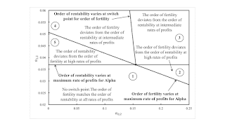
| Figure 2: The Parameter Space for an Example of Extensive Rent |
One can calculate the cost of capital goods at the given rate of profits and the cost of labor inputs for corn-producing processes on each of Type 1 and Type 2 lands. Since coefficients of production are specified per bushel corn produced, the revenues from each of these processes, at a unit level, are the same as the process operated on Type 3 land. Rent is the difference between revenues and non-land costs on Type 1 and Type 2 lands. Rent per acre is plotted in the right pane for Figure 1. The order of rentability is the order of lands by rent per acre. The order of rentability is the same as the order of fertility for any rate of profits below the maximum rate of profits for the given parameters.
The fluke switch point in Figure 1 does not lie on the (inner) wage frontier. The maximum rate of profits for the wage curve for Alpha is the maximum rate of profits for this example. The switch point for the wage curves for the Beta and Gamma techniques is at this maximum rate of profits. Likewise, the rent curves in the right pane in Figure 1 intersect at this maximum rate of profits. As seen in Figure 2, this is another edge case, a fluke that arises in models of extensive rent.
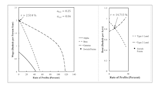
Qualitative properties of the analysis of the choice of technique do not vary within each numbered region. In region 1 in Figure 2, the intersections between the wage and rent curves occur at a rate of profits greater the maximum rate of profits for Alpha. The order of fertility matches the order of rentability. The switch point between the wage curves is at a rate of profits less than the maximum rate of profits in region 2. The order of fertility varies with the rate of profits and deviates from the order of rentability at high rates of profits. Figure 3 illustrates region 3. The intersection between rent curves now also occurs at a rate of profits less than the maximum. In region 4, the intersection between rent curves occurs at a rate of profits less that the rate at which wage curves intersect, in contrast to region 3. In both regions, the orders of fertility and rentability do not match at rates of profits between these intersections. In region 5, the intersection between wage curves occurs at a rate of profits greater than the maximum rate. The orders of fertility and rentability continue to match at rate of profits less than the rate of profits at which rent curves intersect.
| Figure 3: Wage Curves and Rent for Region 3 |
This example illustrates how both the variation of the order of fertility and of the order of rentability with the rate of profits can emerge from perturbations of coefficients of production. It is not necessary for more fertile lands to pay a higher rent. Whether or not these orders match can vary with distribution. Fluke cases specific to models of extensive rent partition the part of the parameter space examined here.
 Heterodox


