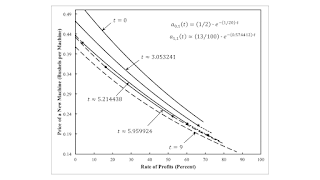
Figure 1: Structural Economic Dynamics of the Price of a New Machine I am not sure that there is any great insight here. But this post depicts the evolution of prices in an example which I have been explaining in two posts. For some parameters, I have found that a shorter economic life of a machine may be associated with a more capital-intensive technique around a switch point. This can occur at both a 'normal' and a 'perverse' switch point. This finding raises difficulties for tradional expositions of Austrian capital theory. In this post, I repeat the specification of technology. Table 1 presents coefficients of production. Corn is both a consumption good and a capital good, insofar as it is an input into all four processes. Corn is also the numeraire. Machines are only capital goods.
Topics:
Robert Vienneau considers the following as important: Austrian School Of Economics, Example in Mathematical Economics, Joint Production
This could be interesting, too:
Robert Vienneau writes Austrian Capital Theory And Triple-Switching In The Corn-Tractor Model
Robert Vienneau writes Double Fluke Cases For Triple-Switching In The Corn-Tractor Model
Robert Vienneau writes The Emergence of Triple Switching and the Rarity of Reswitching Explained
Robert Vienneau writes Recap For A Triple -Switching Example
| Figure 1: Structural Economic Dynamics of the Price of a New Machine |
I am not sure that there is any great insight here. But this post depicts the evolution of prices in an example which I have been explaining in two posts. For some parameters, I have found that a shorter economic life of a machine may be associated with a more capital-intensive technique around a switch point. This can occur at both a 'normal' and a 'perverse' switch point. This finding raises difficulties for tradional expositions of Austrian capital theory.
In this post, I repeat the specification of technology. Table 1 presents coefficients of production. Corn is both a consumption good and a capital good, insofar as it is an input into all four processes. Corn is also the numeraire. Machines are only capital goods. Technology is not yet fully specified in this example, with numerical values undefined for two coefficients of production. The machine does not work with a constant efficiency throughout its physical life. The inputs of seed corn needed to work with the machine increase in agriculture as the machine ages. Labor inputs first increase and then decrease. A one-year old machine is more efficient than both a two-year old and a three-year old machine. Whether a two-year old machine is more efficient than a three-year old machine cannot be determined based on physical data alone. I assume constant returns to scale and free disposal of old machines.
| Input | Industry | Agriculture | ||
| I | II | III | IV | |
| Labor | a0,1 | 39/200 | 117/200 | 39/100 |
| Corn | a1,1 | 39/100 | 141/250 | 117/200 |
| New Machines | 0 | 1 | 0 | 0 |
| 1-Year Old Machines | 0 | 0 | 1 | 0 |
| 2-Year Old Machines | 0 | 0 | 0 | 1 |
| Output | ||||
| Corn | 0 | 1 | 1 | 1 |
| New Machines | 1 | 0 | 0 | 0 |
| 1-Year Old Machines | 0 | 1 | 0 | 0 |
| 2-Year Old Machines | 0 | 0 | 1 | 0 |
I defined the techniques in the previous posts. In the Alpha technique, the machine is run for one year. In Beta, it is run for two years. In Gamma, it is run for its full physical life of three years.
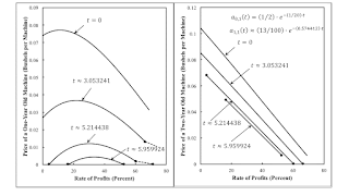
The evolution of the coefficients for production for labor and corn inputs in manufacturing the machine is as noted in Figure 1. I showed previously that, with these specific assumptions, time is partitioned by fluke switch points. Aside from extremes at a time t of 0 and 9, I chose three instants of time, each at the midpoint of one of these partitions. Figures 1 and 2 graph the price of a new machine, one-year old machine, and two-year old machine as functions of the rate of profits at these instants of time.
| Figure 2: Structural Economic Dynamics of the Prices of Old Machines |
As time goes on, the price of production of each vintage machine decreases at any given rate of profits with technical progress in the manufacture of machines. The maximum possible rate of profits, when 'workers live on air', also increases with technical progress.
At the start of time, the Gamma technique is cost-minimizing for any feasible rate of time. This is depicted by the top curve in Figure 1 and both panes of Figure 2. At the end of time, technical progress has made the Alpha technique cost-minimizing for any feasible rate of profits. See the bottom curve in Figure 1. Since the prices of one-year old and two-year old machines are zero for Alpha, no curves for t = 9 appear in Figure 2.
The choice of the economic life of the machine varies with the rate of profits at intermediate times. About when t = 3, the price of a two-year old machine turns negative at a high enough rate of profits at Gamma prices. The machine can still be used in this range if it disposed of after running for two years. At the start of the second year, it is one year old and has a positive price. The Beta technique is cost-minimizing at a high enough rate of profits. At the switch point in which the price of the two-year old machine is zero, the prices of new and one-year old machines are the same for Beta and Gamma techniques. This common price of machines is an illustration of the general result that prices are unique at switch points.
A time around t = 5.214 is an example of reswitching. The price of a one-year old machine is negative, at Gamma and Beta prices, at a rate of profits of zero. Thus, for a low enough rate of profits, the Alpha technique is cost-minimizing. The price of a one-year old machine turns positive at Gamma prices, with an increase in the rate of profits, before it turns positive for Beta prices. A first switch point exists between Alpha and Gamma at a low rate of profits. At a higher rate of profits, the price of a two-year machine becomes zero at Gamma prices. This is the switch point between Beta and Gamma noted in the previous paragraph above. Finally, the price of a one-year old machine becomes negative at Beta prices at a high rate of profits, and Alpha is once again cost-minimizing.
A time around t = 5.96 is a simpler case of reswitching, between Alpha and Gamma. Two switch points exist, and the price of a one-year old machine is zero at Gamma prices at those switch points. The price of a one-year old machine at Beta prices is always negative for all feasible rate of profits.
This analysis demonstrates how examining when prices of production become negative relates to the determination of the cost-minimizing economic life of a machine. At switch points, the price of some old machine is zero.
Depreciation charges fall out of this analysis. Depreciation is the difference in price, at a given rate of profits, of a machine between two years. In the case of a machine of constant efficiency, charges for the cost of machines vary as the value of an annuity lasting for the length of the life of the machine. Modeling the price of a machine as varying as radioactive decay is not a good choice. The example illustrates the more general case of non-constant efficiency. Strangely enough, the machine appreciates from the second year to the third year when the cost-minimizing choice of technique is to run the machine for its full physical life.
 Heterodox


