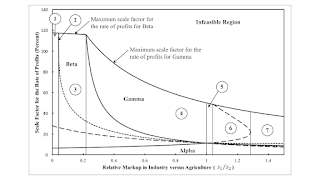
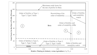
Figure 1: Variation of Technique with Relative Markups "That 'diminishing returns' was not an essential element in the surplus-based theory emerged in Marx's criticisms of Ricardo. Sraffa (1960), in his short chapter on land, the implications of which have yet to be developed, shows how the classical view of rents need not necessarily rest on the conception of 'the law of diminishing returns' or need not suggest necessarily any functional relationship between output and cost, or even presume a unique rank ordering of lands according to productivity. In fact, correcting the classical writers, her shows that differential rents as well as the 'no-rent' land depend upon the rate of profit (or wages)." -- Krishna Bharadwaj (1984) Piero Sraffa: A Tribute Economic and Political Weekly 19 (30-1):
Topics:
Robert Vienneau considers the following as important: Full Cost Prices, rent, Sraffa Effects
This could be interesting, too:
Robert Vienneau writes Three Examples For The Cambridge Capital Controversy
Robert Vienneau writes Variations In An Analysis Of Intensive Rent With One Type Of Land (Part 2/2)
Robert Vienneau writes Variations In An Analysis Of Intensive Rent With One Type Of Land (Part 1/2)
Robert Vienneau writes Variations In Switch Points With Markups In The ‘Corn’ Industry
| Figure 1: Variation of Technique with Relative Markups |
"That 'diminishing returns' was not an essential element in the surplus-based theory emerged in Marx's criticisms of Ricardo. Sraffa (1960), in his short chapter on land, the implications of which have yet to be developed, shows how the classical view of rents need not necessarily rest on the conception of 'the law of diminishing returns' or need not suggest necessarily any functional relationship between output and cost, or even presume a unique rank ordering of lands according to productivity. In fact, correcting the classical writers, her shows that differential rents as well as the 'no-rent' land depend upon the rate of profit (or wages)." -- Krishna Bharadwaj (1984) Piero Sraffa: A Tribute Economic and Political Weekly 19 (30-1): 1236-1235.1.0 Introduction
This example illustrates how the struggle over distribution can be complicated. I start with a fluke case, in which three wage curves intersect at a switch point for a model of competitive capitalism with wage labor and extensive rent.
I assume markup pricing, with a stable ratio of the rate in profits in industry to the rate of profits in agriculture. For each such ratio, consider how the choice of the cost-minimizing technique varies with an exogeneous rate of profits. The wage varies, but so do rents per acre, including even which lands pay rent and which do not, because they are not scarce.
This post demonstrates that the introduction of markup pricing into a model of extensive can result in the reswitching of the order of fertility and the reswitching of the order of rentability.
I think I have demonstrated that one can conduct more research in price theory.
2.0 TechnologyTable 1 presents the technology for the example. The second column shows the inputs of labor, iron, and corn needed to produce a ton of iron. The remaining three columns to the right are the coefficients of production for processes to produce corn. A unit level of operation of a process in agriculture produces a bushel corn and requires an input of one of three types of land, as shown. Constant returns to scale prevail, although the level of operation of the processes producing corn is limited by the available acreage. This example has the same structure as a previous example, with different numbers.
| Input | Industry | |||
| Iron | Corn | |||
| I | II | III | IV | |
| Labor | 1 person-yr. | 0.89965 person-yrs. | 0.60518 person-yr. | 0.58085 person-yr. |
| Type I Land | 0 | 1 acre | 0 | 0 |
| Type II Land | 0 | 0 | 0.98020 acre | 0 |
| Type III Land | 0 | 0 | 0 | 0.38724 acre |
| Iron | 9/20 ton | 1/40 ton | 0.0014882 ton | 0.058085 ton |
| Corn | 2 bushels | 1/10 bushel | 0.45438 bushel | 0.12908 bushel |
The given data also include the land available and the requirements for use. These are such that all three type of land must be at least partially farmed. Specifically, 100 acres of each type of land exist, and net output consists of 300 bushels corn. Three hundred bushels of corn is taken as the numeriare.
Three techniques, Alpha, Beta, and Gamma, can feasibly satisfy requirements for use. In all three techniques, all four processes are operated. One of the types of land is not fully cultivated in each technique. Table 2 displays which type of land is only partially cultivated in each technique. The choice of technique is based on cost-minimization or profit maximization.
| Technique | Land | ||
| Type 1 | Type 2 | Type 3 | |
| Alpha | Partially farmed | Fully farmed | Fully farmed |
| Beta | Fully farmed | Partially farmed | Fully farmed |
| Gamma | Fully farmed | Fully farmed | Partially farmed |
Prices of production are here defined for a given ratio of markups in the industrial and agriculture sectors. The rate of profits in the process producing iron is s1r, while the rate of profits in each of the three processes producing corn is s2r. I call r the scale factor for the rate of profits.
Each of the processes in the technology contributes an equation to the system of equations defining prices of production. The rate of profits is calculated on the value of the capital goods advanced. Rent and wages are paid out of the surplus. Four equations are defined in terms of seven variables, the prices of iron and corn, the rents per acre on each of the three types of land, the wage, and the scale factor for the rate of profits. The coefficients of production and the markups s1 and s2 are taken as given.
Specifying the numeraire removes one degree of freedom. All rents must be non-negative and one type of land must pay no rent. This is the type of land not fully cultivated. This constraint removes another degree of freedom. The system of equations for prices of production has one degree of freedom for this model of markup pricing with extensive rent. This degree of freedom can be expressed as a function showing how the wage decreases with the scale factor for the rate of profits. With the rate of profits somehow specified, the wage, the price of iron, and rent on the scarce land are determined.
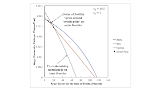
3.0 The Choice of Technique: An Example with Agriculture Having Market PowerFigure 2 illustrates wage curves for the specified markups. Since the ratio s1/s2 is less than unity, this is a case in which agriculture has more market power than industry. For a given scale factor for the rate of profits, the order of fertility is from the type of land associated with the technique with the highest wage curve downwards. The cost minimizing technique corresponds to the wage curve on the inner frontier.
| Figure 2: Wage Curves with Agriculture Having Market Power |
Consider a small scale factor for the rate of profits is such that Alpha is cost-minimizing. If the requirements for use were small enough that they could be satisfied by only farming Type 3 land, Gamma would be cost-minimizing. No land would pay rent and the wage would be as shown on the highest wage curve. With somewhat greater requirements for use, Type 2 land would be taken into cultivation, and the wage would be as shown on the wage curve for Beta. Type 3 land would be fully cultivated and pay a rent. Finally, with the originally postulated requirements for use, Type 1 land is cultivated. In the range for the smallest scale factor for the rate of profits, the order of fertility, from most fertile to least fertile land, is Type 3, Type 2, Type 1.
When Beta is cost-minizing, the order of fertility is Type 3, Type 1, and Type 2 land or Type 1, Type 3, Type 2 land, depending on whether the scale factor for the rate of profits is less than or greater then the scale factor for the rate of profits at the switch point on the outer frontier. For a higher range of the scale factor for the rate of profits, Gamma is cost minimizing, and the order of fertility is Type 1, Type 2, and Type 3 lands.
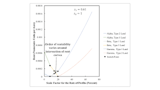
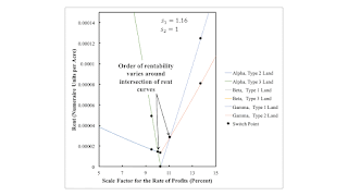
Figure 3 graphs the rent curves for the specified markups. For each switch point for the wage curves, a pair of points, vertically stacked are shown on the graphs. For the switch points on the inner frontier of the wage curves, two rent curves intersect at a rent of zero. For the first such switch point, Type 2 and Type 1 land pay no rent at the switch point. For the switch point between the Beta and Gamma techniques, Type 3 and Type 2 lands pay no rent at the switch point.
| Figure 3: Rent Curves with Agriculture Having Market Power |
The switch point for the intersection on the outer frontier between the Alpha and Gamma wage curves is not striking on the graph of the rent curves. One sees one point on one rent curve for the Beta technique above the other.
The intersection for the two rent curves for the Beta technique occurs at a different scale factor for the rate of profits. It is not a scale factor for the rate of profits for which two wage curves intersect. When Beta is cost minimizing, the order of rentability is Type 3, Type 1, Type 2 for scale factors for the rate of profits less than the scale factor at which the rent curves intersect. For greater scale factors, the order of rentability is Type 1, Type 3, Type 2 when Beta is cost-minimizing.
This example demonstrates that the cost-minimizing technique depends on the scale factor for the rate of profits. The order of fertility of types of lands is not uniquely determined by the cost-minimizing technique. Neither is the order of rentability. And these orders do not need to match. One type of land can obtain more rent per acre than another, even when it is less fertile at the given ratio of markups and scale factor for the rate of profits.
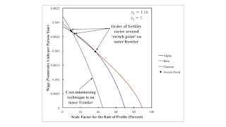
4.0 The Choice of Technique: An Example with Industry Having Market PowerFigure 4 presents another graph of wage curves. Here the ratio of markups, s1/s2, exceeds unity. Industry has more market power than agriculture. The wage curve for the Beta technique is never on the inner frontier, and Beta is never cost-minimizing. This is an example of the reswitching of the order of fertility. When Gamma is cost-minimizing, the order of fertility varies from Type 2, Type 1, Type 3 lands to Type 1, Type 2, Type 3 lands and back.
| Figure 4: Wage Curves with Industry Having Market Power |
Figure 5 shows the rent curves for the given markups. Here the order of rentability varies both when the Alpha technique is cost-minimizing amd when the Gamma technique is cost-minimizing.
| Figure 5: Rent Curves with Industry Having Market Power |
Figure 1, at the top of this post is an attempt to present a synthetic picture of the example. The heavy, solid lines are switch points on the inner frontier of the wage curves and the maximum scale factor for the rate of profits. The cost minimizing technique is labeled. The dashed lines are intersections on the outer frontier of the wage curves. The order of fertility varies across dashed lines. Dotted lines are intersections of rent curves. The order of rentability varies across dotted lines. Dashed and dotted lines are hard to perceive to the right, when industry has more market power than agriculture.
Thin vertical lines parition the ratio of markups. Each vertical line corresponds to a fluke case. Section 3 is a point in region 4. Section 4 is a point in region 6. Figure 6 enlarges the left of the figure, where agriculture has the most market power. For the first fluke case, the rent curves for Type 1 and Type 3 lands, when Beta is cost-minimizing, become tangent at the indicated ratio of markups. The partition between the second and third case is a fluke care where the second intersection for the rent curves for Type 1 and Type 3 lands occurs at the maximum value for the scale factor for the rate of profits. The second region, and the fluke cases bounding it, illustrates that a persistent change in the relative market power among industries can bring about the reswitching of the order of rentability.
| Figure 6: Enlargement of Variation with Relative Markups |
In some sense, the ordinate in Figures 1 and 6 should not have units. I drew the graphs by varying s1, while keeping s2 constant at unity. But one could double both markups, while cutting the scale factor for the rate of profits in half. The graphs would be unchanged.
Anyways, Table 3 summarizes this numeric example. Variations in the cost-minimizing technique, in the order of fertility, and in the order of rentability with the scale factor for the rate of profits are indicated.
| Region | Range | Technique | Order of Fertility | Order of Rentability |
| 1 | 0 ≤ r ≤ r1 | Alpha | Type 3, 2, 1 | Type 3, 2, 1 |
| r1 ≤ r ≤ r2 | Beta | Type 3, 1, 2 | Type 3, 1, 2 | |
| r2 ≤ r ≤ rmax, β | Type 1, 3, 2 | |||
| 2 | 0 ≤ r ≤ r1 | Alpha | Type 3, 2, 1 | Type 3, 2, 1 |
| r1 ≤ r ≤ r2 | Beta | Type 3, 1, 2 | Type 3, 1, 2 | |
| r2 ≤ r ≤ r* | Type 1, 3, 2 | |||
| r* ≤ r ≤ r** | Type 1, 3, 2 | |||
| r** ≤ r ≤ rmax, β | Type 3, 1, 2 | |||
| 3 | 0 ≤ r ≤ r1 | Alpha | Type 3, 2, 1 | Type 3, 2, 1 |
| r1 ≤ r ≤ r2 | Beta | Type 3, 1, 2 | Type 3, 1, 2 | |
| r2 ≤ r ≤ r* | Type 1, 3, 2 | |||
| r* ≤ r ≤ rmax, β | Type 1, 3, 2 | |||
| 4 | 0 ≤ r ≤ r1 | Alpha | Type 3, 2, 1 | Type 3, 2, 1 |
| r1 ≤ r ≤ r2 | Beta | Type 3, 1, 2 | Type 3, 1, 2 | |
| r2 ≤ r ≤ r* | Type 1, 3, 2 | |||
| r* ≤ r ≤ r3 | Type 1, 3, 2 | |||
| r3 ≤ r ≤ rmax, γ | Gamma | Type 1, 2, 3 | Type 1, 2, 3 | |
| 5 | 0 ≤ r ≤ r1 | Alpha | Type 3, 2, 1 | Type 3, 2, 1 |
| r1 ≤ r ≤ r* | Type 2, 3, 1 | |||
| r* ≤ r ≤ r2 | Type 2, 3, 1 | |||
| r2 ≤ r ≤ r** | Gamma | Type 2, 1, 3 | Type 2, 1, 3 | |
| r** ≤ r ≤ r3 | Type 1, 2, 3 | |||
| r3 ≤ r ≤ rmax, γ | Type 1, 2, 3 | |||
| 6 | 0 ≤ r ≤ r1 | Alpha | Type 3, 2, 1 | Type 3, 2, 1 |
| r1 ≤ r ≤ r* | Type 2, 3, 1 | |||
| r* ≤ r ≤ r2 | Type 2, 3, 1 | |||
| r2 ≤ r ≤ r** | Gamma | Type 2, 1, 3 | Type 2, 1, 3 | |
| r** ≤ r ≤ r3 | Type 1, 2, 3 | |||
| r3 ≤ r ≤ r4 | Type 1, 2, 3 | |||
| r4 ≤ r ≤ rmax, γ | Type 2, 1, 3 | |||
| 7 | 0 ≤ r ≤ r1 | Alpha | Type 3, 2, 1 | Type 3, 2, 1 |
| r1 ≤ r ≤ r* | Type 2, 3, 1 | |||
| r* ≤ r ≤ r2 | Type 2, 3, 1 | |||
| r2 ≤ r ≤ r** | Gamma | Type 2, 1, 3 | Type 2, 1, 3 | |
| r** ≤ r ≤ rmax, γ | Type 1, 2, 3 |
The numerical example illustrations complications that can arise in the conflict over the distribution of the surplus among workers, capitalists in various industries, and owners of types of land. I take the coefficients of production as frozen in considering this conflict. That is, I do not consider the conflict over the length of the work day, the intensity with which workers work, the care they must take to prevent waste, the right to urinate on the job, and so on. It is hard to summarize the example. For example, for middling values of the scale factor for the rate of profits, owners of Type 2 land receive no rent if agriculture has somewhat more market power than industry. This possibility disappears when industry has more market power than agriculture. Anyways, this is another example in which obtaining a higher rent per acre can be connected with owning a less productive asset.
The coefficients of production in Table 1 are only approximate. My next step is to pick somewhat 'nicer' fractions' where the fluke three-technique switch point need not occur in the competitive special case.
 Heterodox

