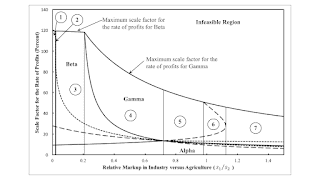
Figure 1: Variation of Technique with Relative Markups1.0 Introduction This is a rewrite of a previous post with somewhat 'nicer' values for coefficients of production. I also expand on it with some observations on absolute rent. As far as I know, these posts are the first explicit presentation in the post-Sraffian tradition of a model of the prices of production with extensive rent and markup pricing. These posts explore the conflict over distribution among workers, capitalists, and landlords. In a model of extensive rent, perturbations of relative market power among industries can create or destroy reswitching of the orders of fertility or of rentability. Extensive rent, called ‘differential rent of the first kind’ by Marx, arises when different types of land are cultivated. The
Topics:
Robert Vienneau considers the following as important: Full Cost Prices, rent, Sraffa Effects
This could be interesting, too:
Robert Vienneau writes Three Examples For The Cambridge Capital Controversy
Robert Vienneau writes Variations In An Analysis Of Intensive Rent With One Type Of Land (Part 2/2)
Robert Vienneau writes Variations In An Analysis Of Intensive Rent With One Type Of Land (Part 1/2)
Robert Vienneau writes Variations In Switch Points With Markups In The ‘Corn’ Industry
| Figure 1: Variation of Technique with Relative Markups |
This is a rewrite of a previous post with somewhat 'nicer' values for coefficients of production. I also expand on it with some observations on absolute rent. As far as I know, these posts are the first explicit presentation in the post-Sraffian tradition of a model of the prices of production with extensive rent and markup pricing.
These posts explore the conflict over distribution among workers, capitalists, and landlords. In a model of extensive rent, perturbations of relative market power among industries can create or destroy reswitching of the orders of fertility or of rentability. Extensive rent, called ‘differential rent of the first kind’ by Marx, arises when different types of land are cultivated. The same commodity, 'corn', is produced on each type of land, with a different mixture of labor and material inputs on each. An industrial commodity, 'iron', is produced in the numerical example explored in this article, thereby ensuring that capital consists of heterogeneous products.
2.0 TechnologyTable 1 presents the technology for the example. The second column shows the inputs of labor, iron, and corn needed to produce a ton of iron. The remaining three columns to the right are the coefficients of production for processes to produce corn. A unit level of operation of a process in agriculture produces a bushel corn and requires an input of one of three types of land, as shown. Constant returns to scale prevail, although the level of operation of the processes producing corn is limited by the available acreage. This example has the same structure as a previous example, with different numbers.
| Input | Industry | |||
| Iron | Corn | |||
| I | II | III | IV | |
| Labor | 1 person-yr. | 9/10 person-yrs. | 6/10 person-yr. | 29/50 person-yr. |
| Type I Land | 0 | 1 acre | 0 | 0 |
| Type II Land | 0 | 0 | 49/50 acre | 0 |
| Type III Land | 0 | 0 | 0 | 2/5 acre |
| Iron | 9/20 ton | 1/40 ton | 3/2000 ton | 29/500 ton |
| Corn | 2 bushels | 1/10 bushel | 9/20 bushel | 13/100 bushel |
In the three processes for producing corn, process III requires more labor per acre of land than process II, and process IV requires even more. Output per acre of land also increases across these three processes. Process III requires less seed corn per acre than process II, and process IV requires even less. Given these contrasts, processes II, III, and IV cannot be ranked by physical efficiency alone. Iron inputs per acre do not even vary monotonically among processes II, III, and IV, further illustrating the need for prices to rank lands by efficiency.
The given data includes the land available and the requirements for use. These are such that all three type of land must be at least partially farmed. Specifically, 100 acres of each type of land exist, and net output consists of 300 bushels corn. Three hundred bushels of corn is taken as the numeraire. The given data are in principle observable at a single moment in time. Different types of land are distinguished by how corn is grown on them. No need exists to imagine marginal adjustments (Gehrke 2021).
Three techniques, Alpha, Beta, and Gamma, can feasibly satisfy requirements for use. In all three techniques, all four processes are operated. One of the types of land is not fully cultivated in each technique (Table 2). The choice of technique is based on cost-minimization or profit maximization.
| Technique | Land | ||
| Type 1 | Type 2 | Type 3 | |
| Alpha | Partially farmed | Fully farmed | Fully farmed |
| Beta | Fully farmed | Partially farmed | Fully farmed |
| Gamma | Fully farmed | Fully farmed | Partially farmed |
Prices of production are here defined for a given ratio of markups in the industrial and agriculture sectors. The rate of profits in the process producing iron is s1r, while the rate of profits in each of the three processes producing corn is s2r. I call r the scale factor for the rate of profits. Prices of production satisfy the following system of equations:
(p1a1,1 + p2a2,1)(1 + s1r) + w a0,1 = p1
(p1a1,2 + p2a2,2)(1 + s2r) + ρ1c1,2 + w a0,2 = p2
(p1a1,3 + p2a2,3)(1 + s2r) + ρ2c2,3 + w a0,3 = p2
(p1a1,4 + p2a2,4)(1 + s2r) + ρ3c3,4 + w a0,4 = p2
I am assuming that wages and rents are paid out of the surplus at the end of the period of production. The relative market power of industry over industry, or vice versa, is expressed by the ratio s1/s2. When this ratio is unity, the equations characterize a competitive capitalist economy.
Each of the processes in the technology contributes an equation to the system of equations defining prices of production. The rate of profits is calculated on the value of the capital goods advanced. Rent and wages are paid out of the surplus. Four equations are defined in terms of seven variables, the prices of iron and corn, the rents per acre on each of the three types of land, the wage, and the scale factor for the rate of profits. The coefficients of production and the markups s1 and s2 are taken as given.
The following equation specifies that the rent on at least one type of land is zero:
ρ1 ρ2 ρ3 = 0
Specifying the numeraire removes one degree of freedom:
300 p2 = 1
All rents must be non-negative and one type of land must pay no rent. This is the type of land not fully cultivated. This constraint removes another degree of freedom. The following equation specifies that the rent on at least one type of land is zero:
ρ1 ρ2 ρ3 = 0
This constraint removes another degree of freedom. The system of equations for prices of production has one degree of freedom for this model of markup pricing with extensive rent. This degree of freedom can be expressed as a function showing how the wage decreases with the scale factor for the rate of profits. With the rate of profits somehow specified, the wage, the price of iron, and rent on the scarce land are determined.
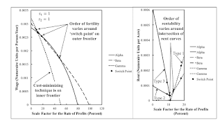
4.0 The Choice of Technique: An Example with Competitive MarketsFigure 2 illustrates wage and rent curves when s1 and s2 are unity. Markets are competitive, and the scale factor for the rate of profits is merely the rate of profits. The cost-minimizing technique corresponds to the wage curve on the inner frontier.
Consider a rate of profits of zero or just barely positive. Alpha is cost-minimizing. If the requirements for use were small enough that they could be satisfied by only farming Type 3 land, a technique with same wage curve as Gamma would be cost-minimizing. No land would pay rent and the wage would be as shown on the highest wage curve. With somewhat greater requirements for use, Type 2 land would be taken into cultivation, and the wage would be as shown on the wage curve for Beta. Type 3 land would be fully cultivated and pay a rent. Finally, with the originally postulated requirements for use, Type 1 land is cultivated. In the range for the smallest rate of profits, the order of fertility, from most fertile to least fertile land, is Type 3, Type 2, Type 1.
| Figure 2: Wage and Rent Curves with Competitive Markets |
Alpha is still cost-minimizing for a rate of profits greater than that at the first intersection on the outer frontier for the wage curves, but smaller than that at the switch point on the inner frontier of the wage curves. For a given rate of profits the order of fertility is from the type of land associated with the technique with the highest wage curve downwards. In this range of the rate of profits, the order of fertility is Type 2, Type 3, Type 1.
This is an example of the reswitching of the order of fertility. When Gamma is cost-minimizing, the order of fertility varies from Type 2, Type 1, Type 3 lands to Type 1, Type 2, Type 3 lands and back. The wage curve for the Beta technique is never on the inner frontier, and Beta is never cost-minimizing.
Rent curves are graphed on the right pane in Figure 2. For each switch point for the wage curves, a pair of points, vertically stacked, are shown on the graph of rent curves. For the switch points on the inner frontier of the wage curves, two rent curves intersect at a rent of zero. Type 1 and Type 3 lands pay no rent at this switch point. The switch points for the intersections on the outer frontier of wage curves are not striking on the graph of the rent curves.
The intersections for the rent curves occur at rates of profits different from those for which wage curves intersect. When Alpha is cost-minimizing, the order of rentability varies from Type 3, Type 2, Type 1 to Type 2, Type 3, Type 1. The order of fertility first matches the order of rentability, then deviates from it at a higher rate of profits, then matches again at a still higher rate of profits. Whether or not the orders of fertility and rentability match also varies with the rate of profits in the range where Gamma is cost-minimizing and Type 3 land pays no rent.
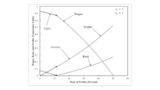
| Figure 3: Distribution of National Income with Competitive Markets |
Given net output and the rate of profits, the levels of operation of each process, the prices of their inputs, and the value of the components of net output are defined. Figure 3 plots total wages, rent, and profits as functions of the rate of profits. Since net output is taken as numeraire, these components add up to unity, whatever the rate of profits. Wages decrease and profits increase with the rate of profits, but rents do not vary monotonically. When Type 1 land is non-scarce, total rents decrease with the rate of profits. When Type 3 land is non-scarce, on the other hand, total rents increase with the rate of profits.
5.0 Perturbing Relative MarkupsThe non-competitive case can differ qualitatively from the competitive case presented in Section 4. In a non-competitive case, with agriculture having sufficient market power, Beta is sometimes cost-minimizing. This is never so in the competitive case. Throughout the range for the scale factor for the rate of profits in which the Alpha technique is cost-minimizing in this non-competitive case, the orders of efficiency and rentability do not vary. The same is true for the range of the scale factor in which Gamma is cost-minimizing. The opposite is true in the competitive case, and sometimes the order of rentability does not match the order of fertility when Alpha or Gamma are cost-minimizing.
One can construct an overall picture of how these changes come about by analyzing the full range of possible ratios of the markup in industry to the markup in agriculture. The heavy, solid lines in Figure 1, at the top of this post, are switch points on the inner frontier of the wage curves and the maximum scale factor for the rate of profits. The cost-minimizing technique is labeled. The dashed lines are intersections on the outer frontier of the wage curves. The order of fertility varies across dashed lines. Dotted lines are intersections of rent curves. The order of rentability varies across dotted lines. Dashed lines are hard to perceive to the right, when industry has more market power than agriculture.
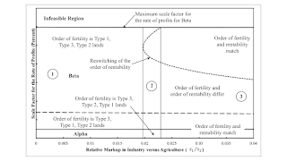
| Figure 4: Enlargement of Variation with Relative Markups |
Thin vertical lines partition the axis for the ratio of markups. Each vertical line corresponds to a fluke case. Figure 4 enlarges the left part of the figure, where agriculture has the most market power. For the first fluke case, the rent curves for Type 1 and Type 3 lands, when Beta is cost-minimizing, become tangent at the indicated ratio of markups. The partition between the second and third region is a fluke case where the second intersection for the rent curves for Type 1 and Type 3 lands occurs at the maximum value for the scale factor for the rate of profits. At the ratio for markups for the third fluke case, the wage curves for Beta and Gamma techniques intersect with a wage of zero. The fourth fluke case is a ratio of markups such that all three wage curves intersect at a single switch point. The rents of all three types of land are zero at that switch point. The fifth fluke case, at a partition between Regions 5 and 6, is such that the wage curves for Alpha and Beta intersect at the maximum scale factor for the Gamma technique. The wage curves for the Alpha and Beta techniques are tangent at a switch point for the ratio of markups at the last fluke case.
Table 3 summarizes this numeric example. Variations in the cost-minimizing technique, in the order of fertility, and in the order of rentability with the scale factor for the rate of profits are indicated. In Region 1, agriculture has the most extreme level of market power over industry. The wage curve for Alpha intersects the wage curve for Beta on the inner frontier and then the wage curve for Gamma on the outer frontier. The rent curves do not intersect in the appropriate ranges of the scale factor for the rate of profits. The order of rentability only varies with the cost-minimizing technique.
| Region | Range | Technique | Order of Fertility | Order of Rentability |
| 1 | 0 ≤ r ≤ r1 | Alpha | Type 3, 2, 1 | Type 3, 2, 1 |
| r1 ≤ r ≤ r2 | Beta | Type 3, 1, 2 | Type 3, 1, 2 | |
| r2 ≤ r ≤ rmax, β | Type 1, 3, 2 | |||
| 2 | 0 ≤ r ≤ r1 | Alpha | Type 3, 2, 1 | Type 3, 2, 1 |
| r1 ≤ r ≤ r2 | Beta | Type 3, 1, 2 | Type 3, 1, 2 | |
| r2 ≤ r ≤ r* | Type 1, 3, 2 | |||
| r* ≤ r ≤ r** | Type 1, 3, 2 | |||
| r** ≤ r ≤ rmax, β | Type 3, 1, 2 | |||
| 3 | 0 ≤ r ≤ r1 | Alpha | Type 3, 2, 1 | Type 3, 2, 1 |
| r1 ≤ r ≤ r2 | Beta | Type 3, 1, 2 | Type 3, 1, 2 | |
| r2 ≤ r ≤ r* | Type 1, 3, 2 | |||
| r* ≤ r ≤ rmax, β | Type 1, 3, 2 | |||
| 4 | 0 ≤ r ≤ r1 | Alpha | Type 3, 2, 1 | Type 3, 2, 1 |
| r1 ≤ r ≤ r2 | Beta | Type 3, 1, 2 | Type 3, 1, 2 | |
| r2 ≤ r ≤ r* | Type 1, 3, 2 | |||
| r* ≤ r ≤ r3 | Type 1, 3, 2 | |||
| r3 ≤ r ≤ rmax, γ | Gamma | Type 1, 2, 3 | Type 1, 2, 3 | |
| 5 | 0 ≤ r ≤ r1 | Alpha | Type 3, 2, 1 | Type 3, 2, 1 |
| r1 ≤ r ≤ r* | Type 2, 3, 1 | |||
| r* ≤ r ≤ r2 | Type 2, 3, 1 | |||
| r2 ≤ r ≤ r** | Gamma | Type 2, 1, 3 | Type 2, 1, 3 | |
| r** ≤ r ≤ r3 | Type 1, 2, 3 | |||
| r3 ≤ r ≤ rmax, γ | Type 1, 2, 3 | |||
| 6 | 0 ≤ r ≤ r1 | Alpha | Type 3, 2, 1 | Type 3, 2, 1 |
| r1 ≤ r ≤ r* | Type 2, 3, 1 | |||
| r* ≤ r ≤ r2 | Type 2, 3, 1 | |||
| r2 ≤ r ≤ r** | Gamma | Type 2, 1, 3 | Type 2, 1, 3 | |
| r** ≤ r ≤ r3 | Type 1, 2, 3 | |||
| r3 ≤ r ≤ r4 | Type 1, 2, 3 | |||
| r4 ≤ r ≤ rmax, γ | Type 2, 1, 3 | |||
| 7 | 0 ≤ r ≤ r1 | Alpha | Type 3, 2, 1 | Type 3, 2, 1 |
| r1 ≤ r ≤ r* | Type 2, 3, 1 | |||
| r* ≤ r ≤ r2 | Type 2, 3, 1 | |||
| r2 ≤ r ≤ r** | Gamma | Type 2, 1, 3 | Type 2, 1, 3 | |
| r** ≤ r ≤ rmax, γ | Type 1, 2, 3 |
Region 2, and the fluke cases bounding it, illustrates that a persistent change in the relative market power among industries can bring about the reswitching of the order of rentability. The rent curves for Type 1 and Type 3 land intersect twice in the range of the scale factor of profits in which Beta is cost-minimizing. The rent curves for both types of land are increasing functions of the scale factor in this range.
The rent curve for Type 3 land becomes downward-sloping in Region 3. It is not always monotone. The order of rentability at the highest range of the scale factor for the rate of profits in Region 2 has disappeared in Region 3. With some thought, one can see how the variations between regions in the ranges of the scale factor for the cost-minimizing technique, the order of fertility, and the order of rentability relate to the fluke cases dividing these regions. The range of the scale factor in which Beta is cost-minimizing has disappeared in Region 5, after the switch point at which all three wage curves intersect. Switch points between Alpha and Beta and between Beta and Gamma are thenchforth on the outer wage frontier and are the occasion of a change in the order of fertility. Region 6 is an example of the reswitching of the order of fertility, and is illustrated in Section 4 with the competitive case. In Region 7, the last in the table, the order of fertility does not vary when Gamma is cost-minimizing.
6.0 ConclusionThe numerical example illustrates complications that can arise in the conflict over the distribution of the surplus among workers, capitalists in various industries, and owners of types of land. I take the coefficients of production as frozen in considering this conflict. That is, I do not consider the conflict over the length of the working day, the intensity with which workers work, the care they must take to prevent waste, the right to urinate on the job, and so on. Nor do I consider some conflicts between capitalists and landlords, outside of distribution. For example, landlords would like leases as short as possible so as to be able to raise rents for more-or-less permanent improvements brought about by the capitalists, while the capitalists would like longer rents to prevent this outcome.
The model illustrated above is one in which relative markups are given. It demonstrates that in the competitive case, the order of fertility of lands can vary with the rate of profits, where the rate of profits is taken as given from outside the model. The order of fertility can vary both with and without the cost-minimizing technique varying. The order of lands from high rent to low rent lands also varies, in general, with the rate of profits. One may find that ownership of one type of asset provides greater returns than another, even though the latter asset is more efficient at the going rate of profits.
Persistent differences in markups among industries does not alter these conclusions, but does provide the possibility of qualitative and quantitative variation in details. In the example, if agriculture has sufficient market power over industry, the example no longer exhibits a reswitching of the order of fertility. A range of the scale factor for the rate of profits emerges in which type 2 land no longer obtains a rent. An even further increase in the market power of agriculture can lead to the appearance and the disappearance of the reswitching of the order of rentability
No simple picture emerges from this analysis. The workers can only obtain a larger share of the surplus product if the capitalists get less. Whether or not the landlords are able to obtain a larger share with either an increased rate of profits or increased market power for some sectors varies
 Heterodox


