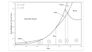
Figure 1: Variation in the Maximum Wage and the Cost-Minimizing Technique with Time This post presents an example in which some coefficients of production vary from those in example. Reswitching, capital reversing, and the reverse substitution of labor do not arise in this example. Table 1 shows the coefficients of production for this example. The labor coefficients vary identically with the the labor coefficients in the previous example. a2,1(a), a3,1(a), a2,1(b), a3,1(b), a1,2(c), a3,2(c), and a1,2(d) are all larger in this example. Table 1: The Technology InputIronIndustrySteelIndustryCornIndustryabcdefLabor(15/2) e-φt32 e-σt(13/2) e-φt60 e-σt(15/2) e-φt55 e-σtIron1/62/51/201/1010Steel1/201/201/43/1001/4Corn1/151/151/15000 Table 2 repeats the definition of the techniques of
Topics:
Robert Vienneau considers the following as important: Example in Mathematical Economics, Sraffa Effects
This could be interesting, too:
Robert Vienneau writes Austrian Capital Theory And Triple-Switching In The Corn-Tractor Model
Robert Vienneau writes Double Fluke Cases For Triple-Switching In The Corn-Tractor Model
Robert Vienneau writes The Emergence of Triple Switching and the Rarity of Reswitching Explained
Robert Vienneau writes Recap For A Triple -Switching Example
| Figure 1: Variation in the Maximum Wage and the Cost-Minimizing Technique with Time |
This post presents an example in which some coefficients of production vary from those in example. Reswitching, capital reversing, and the reverse substitution of labor do not arise in this example.
Table 1 shows the coefficients of production for this example. The labor coefficients vary identically with the the labor coefficients in the previous example. a2,1(a), a3,1(a), a2,1(b), a3,1(b), a1,2(c), a3,2(c), and a1,2(d) are all larger in this example.
| Input | Iron Industry | Steel Industry | Corn Industry | |||
| a | b | c | d | e | f | |
| Labor | (15/2) e-φt | 32 e-σt | (13/2) e-φt | 60 e-σt | (15/2) e-φt | 55 e-σt |
| Iron | 1/6 | 2/5 | 1/20 | 1/10 | 1 | 0 |
| Steel | 1/20 | 1/20 | 1/4 | 3/10 | 0 | 1/4 |
| Corn | 1/15 | 1/15 | 1/15 | 0 | 0 | 0 |
Table 2 repeats the definition of the techniques of production. As in the previous example, the Alpha and Theta techniques each undergo Harrod-neutral technical progress.
| Technique | Processes |
| Alpha | a, c, e |
| Beta | a, c, f |
| Gamma | a, d, e |
| Delta | a, d, f |
| Epsilon | b, c, e |
| Zeta | b, c, f |
| Eta | b, d, e |
| Theta | b, d, f |
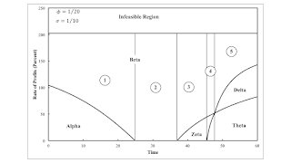
As usual, prices of production are defined for each moment in time. Given the wage or the rate of profits, one can find the cost-minimizing technique. Figure 1, at the top of this post, and Figure 2 depict how the dependence of the cost-minimizing technique on distribution varies with time. These graphs are drawn for the specified rate of technical progress. The variation of the cost-minimizing technique with distribution is invariant in each numbered region, although the specific rate of profits, for example, at which a switch point occurs does vary.
| Figure 2: Variation in the Maximum Rate of Profits and the Cost-Minimizing Technique with Time |
At the maximum rate of profits, the wage is zero. Variations in labor coefficients do not matter. In this case, the Beta technique remains cost-minimizing for all time at a wage of zero. The cost-minimizing technique at the maximum wage varies from Alpha to Theta, as the pure technique with the faster growth in technical progress becomes dominant. Beta and Theta vary in the iron-producing and steel-producing processes. Ultimately, at the extreme right of the graphs, two switch points exist as distribution varies.
I guess these two examples illustrate general properties of Harrod-neutral technical progress in the case where all techniques require the production of the same commodities and all of these commodities are basic in the sense of Sraffa. Fluke cases will arise over time. So-called 'perverse' switch points need not arise, but can.
 Heterodox


