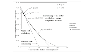
Figure 1: Choice of Technique with Extensive Rent and Competitive Markets1.0 Introduction I am making some slow progress on recreating past posts. For variation, I here take the wage as given. If I write this up more formally, I intend not to try to relate it to Marx's concept of absolute rent. The point is to illustrate the following comment with long-lasting variations in market power between industry and agriculture: "The complexity of the outcomes with the potential existence of conflict or concordance among the three major economic categories (earners of wages, profits, and rents) profoundly modifies the traditional analysis of profits and wages." -- Alberto Quadrio Curzio and Fausta Pellizzari. Rent, Resources, Technologies, Springer,2010: 34. This story illustrates how the
Topics:
Robert Vienneau considers the following as important: rent
This could be interesting, too:
Robert Vienneau writes Variations In An Analysis Of Intensive Rent With One Type Of Land (Part 2/2)
Robert Vienneau writes Variations In An Analysis Of Intensive Rent With One Type Of Land (Part 1/2)
Robert Vienneau writes Intensive Rent With Two Types Of Land
Robert Vienneau writes Intensive Rent And The Order Of Rentability
| Figure 1: Choice of Technique with Extensive Rent and Competitive Markets |
I am making some slow progress on recreating past posts. For variation, I here take the wage as given.
If I write this up more formally, I intend not to try to relate it to Marx's concept of absolute rent. The point is to illustrate the following comment with long-lasting variations in market power between industry and agriculture:
"The complexity of the outcomes with the potential existence of conflict or concordance among the three major economic categories (earners of wages, profits, and rents) profoundly modifies the traditional analysis of profits and wages." -- Alberto Quadrio Curzio and Fausta Pellizzari. Rent, Resources, Technologies, Springer,2010: 34.
This story illustrates how the owner of Type II land is affected by the distribution between wages and profits, depending on the degree of market power between industry and agriculture. Under competitive markets in the example, this owner receives a rent, no matter what the distribution between wage and profits. With a large enough relative markup in agriculture, as compared with industry, they receive zero rents for some distributions between wages and profits. I also illustrate two fluke cases for relative markups.
2.0 Technology and EndowmentsTable 1 presents the technology for the example. The second column shows the inputs of labor, iron, and corn needed to produce a ton of iron. The remaining three columns to the right are the coefficients of production for processes to produce corn. A unit level of operation of a process in agriculture produces a bushel corn and requires an input of one of three types of land, as shown. Constant returns to scale prevail, although the level of operation of the processes producing corn is limited by the available acreage.
| Input | Industry | |||
| Iron | Corn | |||
| I | II | III | IV | |
| Labor | 1 person-yr. | 9/10 person-yrs. | 6/10 person-yr. | 29/50 person-yr. |
| Type 1 Land | 0 | 1 acre | 0 | 0 |
| Type 2 Land | 0 | 0 | 49/50 acre | 0 |
| Type 3 Land | 0 | 0 | 0 | 2/5 acre |
| Iron | 9/20 ton | 1/40 ton | 3/2000 ton | 29/500 ton |
| Corn | 2 bushels | 1/10 bushel | 9/20 bushel | 13/100 bushel |
In the three processes for producing corn, process III requires more labor per acre of land than process II, and process IV requires even more. Output per acre of land also increases across these three processes. Process III requires less seed corn per acre than process II, and process IV requires even less. Given these contrasts, processes II, III, and IV cannot be ranked by physical efficiency alone. Iron inputs per acre do not even vary monotonically among processes II, III, and IV, further illustrating the need for prices to rank lands by efficiency.
I take the numeraire as a commodity basket consisting of 1 ton iron and 1 bushel corn.
The given data includes the land available and the requirements for use. These are such that all three type of land must be at least partially farmed. The given data are in principle observable at a single moment in time. Different types of land are distinguished by how corn is grown on them. No need exists to imagine marginal adjustments
Three techniques, Alpha, Beta, and Gamma, can feasibly satisfy requirements for use. In all three techniques, all four processes are operated. One of the types of land is not fully cultivated in each technique (Table 2). The choice of technique is based on cost-minimization or profit maximization.
| Technique | Land | ||
| Type 1 | Type 2 | Type 3 | |
| Alpha | Partially farmed | Fully farmed | Fully farmed |
| Beta | Fully farmed | Partially farmed | Fully farmed |
| Gamma | Fully farmed | Fully farmed | Partially farmed |
Prices of production are here defined for a given ratio of markups in the industrial and agriculture sectors. The rate of profits in the process producing iron is s1r, while the rate of profits in each of the three processes producing corn is s2r. I call r the scale factor for the rate of profits. Prices of production satisfy the following system of equations:
(p1a1,1 + p2a2,1)(1 + s1r) + w a0,1 = p1
(p1a1,2 + p2a2,2)(1 + s2r) + ρ1c1,2 + w a0,2 = p2
(p1a1,3 + p2a2,3)(1 + s2r) + ρ2c2,3 + w a0,3 = p2
(p1a1,4 + p2a2,4)(1 + s2r) + ρ3c3,4 + w a0,4 = p2
I am assuming that wages and rents are paid out of the surplus at the end of the period of production. The relative market power of industry over agriculture, or vice versa, is expressed by the ratio s1/s2. When this ratio is unity, the equations characterize a competitive capitalist economy. Today, I experiment with assuming markups lie on a simplex:
s1 + s2 = 1
Each of the processes in the technology contributes an equation to the system of equations defining prices of production. The rate of profits is calculated on the value of the capital goods advanced. Rent and wages are paid out of the surplus. Four equations are defined in terms of seven variables, the prices of iron and corn, the rents per acre on each of the three types of land, the wage, and the scale factor for the rate of profits. The coefficients of production and the markups s1 and s2 are taken as given.
Specifying the numeraire removes one degree of freedom:
p1 + p2 = 1
All rents must be non-negative and one type of land must pay no rent. This is the type of land not fully cultivated. The following equation specifies that the rent on at least one type of land is zero:
ρ1 ρ2 ρ3 = 0
This constraint removes another degree of freedom. The system of equations for prices of production has one degree of freedom for this model of markup pricing with extensive rent. This degree of freedom can be expressed as a function showing how the wage decreases with the scale factor for the rate of profits, or vice versa. With the wage somehow specified, the rate of profits in industry and agriculture, the price of iron, and rent on the scarce land are determined.
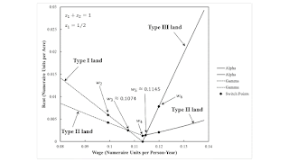
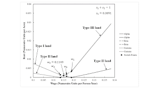
4.0 The Choice of Technique: An Example with Competitive MarketsFigure 1 illustrates wage curves when s1 and s2 are 1/2. Markets are competitive. The cost-minimizing technique corresponds to the wage curve on the inner frontier. Figure 2 illustrates the corresponding rent curves.
| Figure 2: Order of Rentability with Competitive Markets |
Consider a wage of zero or just barely positive. Beta is cost-minimizing. If the requirements for use were small enough that they could be satisfied by only farming Type 2 land, a technique with same wage curve as Beta would be cost-minimizing. No land would pay rent, and the scale fator for the rate of profits would be as shown on the right-most wage curve. With somewhat greater requirements for use, Type 1 land would be taken into cultivation, and the scale factor would be as shown on the wage curve for Alpha. Type 2 would be fully cultivated and pay a rent. Finally, with the originally postulated requirements for use, Type 3 land is cultivated. In the range for the smallest wage, the order of fertility, from most fertile to least fertile land, is Type 2, Type 1, Type 3. The order of fertility is also known as the order of efficiency.
The order of efficiency, for a wage of zero and competitive markets, also orders techniques in decreasing order of the maximum rate of growth. Since land of each type is limited in quantity, the maximum rate of growth must decline, without innovatin.
This is an example of the reswitching of the order of efficiency. When Gamma is cost-minimizing, the order of efficiency varies from Type 2, Type 1, Type 3 lands to Type 1, Type 2, Type 3 lands and back. The inner frontier shows the cost-minimizing technique for this example. The intersections of the wage curves on the outer frontier show variations in the order of efficiency. The wage curve for the Beta technique is never on the inner frontier, and Beta is never cost-minimizing.
The intersections for the rent curves occur at wages different from those for which wage curves intersect. When Gamma is cost-minimizing, the order of rentability varies from Type 1, Type 2, Type 3 to Type 2, Type 1, Type 3. The order of efficiency first deviates from the order of rentability, then matches at a higher wage, deviates at an even higher wage, and matches again at a still higher wage. Whether or not the orders of efficiency and rentability match also varies with the wage in the range where Alpha is cost-minimizing and Type 1 land pays no rent.
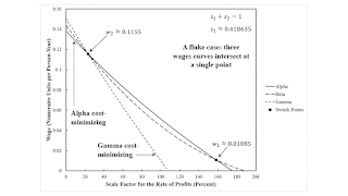
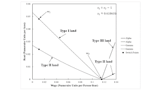
5.0 A Three-Technique Fluke Switch PointSuppose the relative markup in industry is lower. Figures 3 and 4 show the wage and rent curves for a fluke case, in which all three rent curves intersect at a single point. Under Gamma, the order of efficiency, at a wage of zero, starts at Type 2, 1, and 3 lands. The order of rentability, being Type 1, 2, and 3 lands, differs. At a higher wage, the order of efficiency changes, and then matches the order of rentability. When Alpha is cost-minimizing, the orders of efficiency and rentability match. They are both Type 3, 2, and 1 lands.
| Figure 3: Choice of Technique for Three-Technique Fluke Case |
| Figure 4: Order of Rentability for Three-Technique Fluke Case |
I suppose the most interesting aspect of this example, other than its fluke property, is that the switch point for the order of efficiency at the low wage w1 would not exist, in some sense, if the scale factor was taken as given. The scale factor for the rate of profits for this switch point exceeds the maximum scale factor for the Gamma technique.
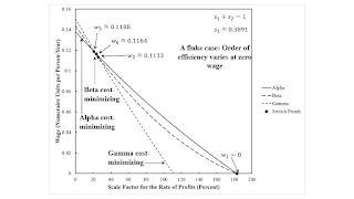
6.0 A Fluke Switch Point with a Variation in the Order of Efficiency at a Wage of ZeroI next want to consider an even lower markup in industry, for another fluke case. A switch point for the order of efficiency exists in Figure 5 on the axis for the scale factor for the rate of profits. Figure 6 shows the corresponding rent curves.
| Figure 5: Choice of Technique for Fluke Case for Order of Efficiency |
| Figure 6: Order of Rentability for Fluke Case for Order of Efficiency |
When Gamma is cost-minimizing at a positive wage, the orders of efficiency and of rentability are Type 1, 2, and 3 lands.
When Beta is cost-minimizing, the orders of efficiency and rentability initially match, with a order of Type 1, 3, and 2 lands. At a higher wage, the order of rentability changes, so they do not match. At an even higher wage, the order of efficiency changes, so the orders once again match, with Beta cost-minimizing.
Alpha is cost-minimizing at the highest range of feasible wages. The orders of efficiency and rentability match, with an order of Type 3, 2, and 1 lands.
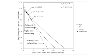
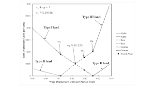
7.0 An Example with Higher Market Power in AgricultureFinally, I want to consider a non-fluke case, with an even lower markup in industry. Figures 7 and 8 show the wage curves and rent curves here. The comments about the orders of efficiency and rentability in the previous section apply, with the exception that the switch point at a wage of zero and disappeared below the axis for the scale factor for the rate of profits.
| Figure 7: Choice of Technique for Example with Market Power for Agriculture |
| Figure 8: Order of Rentability for Example with Market Power for Agriculture |
I like that the orders of efficiency and rentability totally reverse, from the lowest to the highest wage.
More qualitative changes in the analyhsis of the choice of technique, including fluke cases, arise for even lower relative markups in industry. But I want to stop here, where the reswitching of the order of efficiency has vanished and Type 2 land obtains no rent for some intermediate range of the wage.
8.0 ConclusionOne can see that the owners of Type 2 land care about competitive forces among capitalists, and the struggle between the workers and the capitalists. If capitalists in agriculture are able to impose lasting barriers to entry, as compared to capitalists in industry, the struggle over the wage can leave them with no rent at all. Furthermore, the specific level of rents per acre, for all types of land, varies at specific wages, depending on the struggle among capitalists. The order of efficiency can vary from the order of lands from the highest rate of growth to the lowest, even at a wage of zero, depending on the struggle among capitalists. I can expand the above write-up to include one of my one-dimension diagrams.
I draw heavily on the work of Alberto Quadrio Curzio in this post. He looked deeply into the theory of rent in post-Sraffian price theory. The book, Resources, Production, and Structural Dynamics (edited by Mauro L. Baranzini, Claudia Rotondi, and Roberto Scazzieri) is dedicated to him. It contains a lot that differs from this kind of formal analysis, considering institutions for fostering innovation to overcome resources scarcities and so on.
 Heterodox

