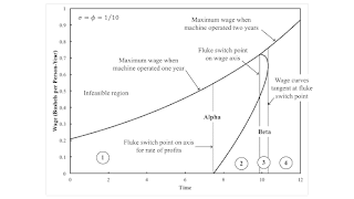
Figure 1: Variation in the Economic Life of a Machine with Technical Progress This post varies the coefficients of production in an example from Bertram Schefold. I wanted to have 'nice' fractions at a time of zero. Qualitatively, this looks like a previous post. Reviewers for a recent rejection of an article with another fixed capital example objected to this type of model. I need to relate technical progress to a well-known type (Harrod-neutral, Marx-biased, or whatever) or produce some evidence that this sort of modeling is reasonable. Table 1 presents the technology for this example. Machines and corn are produced in this economy. Corn is the only consumption good. New machines are produced from inputs of labor and corn. Corn is produced from inputs of labor, corn, and machines.
Topics:
Robert Vienneau considers the following as important: Example in Mathematical Economics, Sraffa Effects
This could be interesting, too:
Robert Vienneau writes Austrian Capital Theory And Triple-Switching In The Corn-Tractor Model
Robert Vienneau writes Double Fluke Cases For Triple-Switching In The Corn-Tractor Model
Robert Vienneau writes The Emergence of Triple Switching and the Rarity of Reswitching Explained
Robert Vienneau writes Recap For A Triple -Switching Example
| Figure 1: Variation in the Economic Life of a Machine with Technical Progress |
This post varies the coefficients of production in an example from Bertram Schefold. I wanted to have 'nice' fractions at a time of zero. Qualitatively, this looks like a previous post.
Reviewers for a recent rejection of an article with another fixed capital example objected to this type of model. I need to relate technical progress to a well-known type (Harrod-neutral, Marx-biased, or whatever) or produce some evidence that this sort of modeling is reasonable.
Table 1 presents the technology for this example. Machines and corn are produced in this economy. Corn is the only consumption good. New machines are produced from inputs of labor and corn. Corn is produced from inputs of labor, corn, and machines. A machine can be worked for two years. After the end of the first year of its working life, it is known as an old machine. I assume each process requires a year to complete and exhibits constant returns to scale.
| Input | Process | ||
| (I) | (II) | (III) | |
| Labor | (7/25) e- σ t | 3 e- φ t | (14/5) e- φ t |
| Corn | (4/25) e- σ t | (4/25) e- φ t | (2/3) e- φ t |
| New Machines | 0 | 1 | 0 |
| Old Machines | 0 | 0 | 1 |
| Outputs | |||
| Corn | 0 | 1 | 1 |
| New Machines | 1 | 0 | 0 |
| Old Machines | 0 | 1 | 0 |
The managers of firms need not run the machine for two years. They could discard the machine after only one year. (I assume free disposal.) I call Alpha the technique in which the machine is run for one year, and Beta the technique in which the machine is run for its full physical year of two years. The managers will be cost-minimizing if they run the machine for only one year if the price of an old machine is negative. Prices are found as prices of production, with an external specification of the wage or the rate of profits.
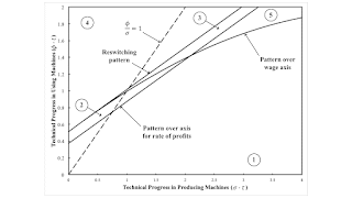
Figure 1 above and Table 2 below illustrate the analysis of the choice of technique. Until time reaches the pattern over the axis for the rate of profits, it is cost-minimizing to operate the machine for only one year. In Region 2, the machine is operated for two years when wages are low, and for one year when wages are higher. Region 3 is an example of reswitching. Eventually, it is cost-minimizing to operate the machine for two years, for all feasible wages.
| Region | Switch Points | Cost-Minimizing Techniques |
| 1 | None | Alpha |
| 2 | One | Beta, Alpha |
| 3 | Two | Beta, Alpha, Beta |
| 4 | None | Beta |
| 5 | One | Alpha, Beta |
Figure 2 partitions the parameter space such that the characteristics of the variations in the choice of technique technique do not vary within each region. Each region is bounded by thick (non-dotted) lines. Suppose that technical progress in producing and using machines is steady. That is, σ and φ have some fixed values. The dotted line in Figure 2 illustrates a path in logical time for such a thought experiment. The 45 degree line corresponds to the case in which σ and φ are equal, as in Figure 1. The numbering of the regions in Figures 1 and 2 and in Table 2 correspond.
| Figure 2: A Parameter Space |
Stepping through this example does not provide any qualitative differences from previous posts. Reswitching in models of fixed capital can be manifested as the return of a period of truncation. Around a switch point, a lower wage need not be associated with greater employment for a given net output. And so on.
 Heterodox


