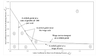
Figure 1: A Larger Parameter Space This post is an expansion on the first example here. It presents shortly a more comprehensive analysis of the variation in the choice of technique in the example of circulating capital in Section 2. Local perturbations of two coefficients of production are examined there. Figure 1 partitions a larger part of the space defined by these two coefficients of production. Table 1 exhibits how the cost-minimizing technique varies with the rate of profits in each region. Table 3: Ranges of the Rate of Profits by Region RegionRangeTechniqueNotes10 ≤ r ≤ r1BetaReverse substitution of labor at switch point.r1 ≤ r ≤ rα,maxAlpha20 ≤ r ≤ r1BetaSwitch point is 'non-perverse'.r1 ≤ r ≤ rα,maxAlpha30 ≤ r ≤ rβ,maxBetaNo switch point.40 ≤ r ≤ rβ,maxBetaNo switch point.50
Topics:
Robert Vienneau considers the following as important:
This could be interesting, too:
Robert Vienneau writes Austrian Capital Theory And Triple-Switching In The Corn-Tractor Model
Mike Norman writes The Accursed Tariffs — NeilW
Mike Norman writes IRS has agreed to share migrants’ tax information with ICE
Mike Norman writes Trump’s “Liberation Day”: Another PR Gag, or Global Reorientation Turning Point? — Simplicius
| Figure 1: A Larger Parameter Space |
This post is an expansion on the first example here. It presents shortly a more comprehensive analysis of the variation in the choice of technique in the example of circulating capital in Section 2. Local perturbations of two coefficients of production are examined there. Figure 1 partitions a larger part of the space defined by these two coefficients of production. Table 1 exhibits how the cost-minimizing technique varies with the rate of profits in each region.
| Region | Range | Technique | Notes |
| 1 | 0 ≤ r ≤ r1 | Beta | Reverse substitution of labor at switch point. |
| r1 ≤ r ≤ rα,max | Alpha | ||
| 2 | 0 ≤ r ≤ r1 | Beta | Switch point is 'non-perverse'. |
| r1 ≤ r ≤ rα,max | Alpha | ||
| 3 | 0 ≤ r ≤ rβ,max | Beta | No switch point. |
| 4 | 0 ≤ r ≤ rβ,max | Beta | No switch point. |
| 5 | 0 ≤ r ≤ r1 | Alpha | Switch point is 'non-perverse'. |
| r1 ≤ r ≤ rβ,max | Beta | ||
| 6 | 0 ≤ r ≤ r1 | Alpha | Reswitching. Second switch point exhibits capital-reverseing and the reverse substitution of labor. |
| r1 ≤ r ≤ r2 | Beta | ||
| r1 ≤ r ≤ rα,max | Alpha | ||
| 7 | 0 ≤ r ≤ rα,max | Alpha | No switch point. |
Section 2 in the previous focuses on regions 1, 2, 3, and 4. Region 3 and 4 differ in that in region 4, the wage curves intersect at a negative rate of profits greater than -100 percent. This post presents an analysis, in a model of fixed capital, much like the fluke switch point associated with the intersections of the partitions between regions 1, 6, and 7. Does checking how the variation of the analysis of the cost-minimizing technique among regions, summarized in Table 1, relates to the fluke cases defining the partitions in Figure 1 clarify that variation? Perturbations of coefficients of production, in this example of circulating capital, illustrate how reswitching can emerge, as well as the emergence of the reverse substitution of labor.
 Heterodox

