When Marx’s theory of value is interpreted in a simultaneist way, it is relatively easy to calculate the ‘monetary expression of labor time’ (or MELT). It is simply new value added, measured in monetary terms, divided by productive employment. If it were not for the ‘productive’/’unproductive’ distinction, the simultaneist MELT could readily be calculated from the National Accounts as the ratio of Net Domestic Product at current prices to Total Employment. Retaining the productive/unproductive dichotomy complicates matters somewhat, because it is then necessary to exclude unproductive activity from the calculations, but no other hurdles appear to be present. There is an additional complication when it comes to measuring the temporal MELT. The temporal MELT is the appropriate measure if
Topics:
peterc considers the following as important: Economics
This could be interesting, too:
Lars Pålsson Syll writes Schuldenbremse bye bye
Lars Pålsson Syll writes What’s wrong with economics — a primer
Lars Pålsson Syll writes Krigskeynesianismens återkomst
Lars Pålsson Syll writes Finding Eigenvalues and Eigenvectors (student stuff)
When Marx’s theory of value is interpreted in a simultaneist way, it is relatively easy to calculate the ‘monetary expression of labor time’ (or MELT). It is simply new value added, measured in monetary terms, divided by productive employment. If it were not for the ‘productive’/’unproductive’ distinction, the simultaneist MELT could readily be calculated from the National Accounts as the ratio of Net Domestic Product at current prices to Total Employment. Retaining the productive/unproductive dichotomy complicates matters somewhat, because it is then necessary to exclude unproductive activity from the calculations, but no other hurdles appear to be present.
There is an additional complication when it comes to measuring the temporal MELT. The temporal MELT is the appropriate measure if Marx’s theory of value is interpreted in a temporal way (as in the ‘temporal single-system interpretation’ or TSSI). The difficulty is due to the fact that the end-of-period MELT (the ‘output MELT’) depends on the start-of-period MELT (the ‘input MELT’). The question becomes how to obtain a measure of an output MELT before we have a measure of an input MELT. It is necessary somehow to approximate, with decent accuracy, the MELT of one period without knowing the previous MELT. If we can do this at least once, then the estimated MELT of that period can become the input MELT of the subsequent period, and from then on we will always have an input MELT to enable the direct calculation of the next output MELT. It will also be possible to work backwards, calculating an earlier MELT from a later one. The purpose of this post is to arrive at a method for approximating a temporal MELT, without knowledge of a prior MELT, while being confident that the estimate will have a decent degree of accuracy.
The challenge is made clear by inspecting a direct formula for the temporal MELT. Initially we are just concerned with period t, which begins at time t and ends at time t+1. The output MELT (mt+1) depends upon the input MELT (mt):
Time subscripts t and t+1 refer to times t and t+1, respectively. The absence of a subscript indicates a process that occurs over the entire period, in this case productive employment L. In some contexts, when dealing with multiple periods, it will be necessary to attach a subscript to processes as well. For period t, the subscript would be t,t+1 to indicate that the process continues throughout the entire period, from beginning to end.
In principle, all but one variable on the right-hand side of (1) can be measured. L, as already mentioned, is total productive employment. $ct is the monetary value of inputs transferred to final output, including wear and tear on plant and equipment. It is the monetary measure of constant capital. $TPt+1 is the monetary value of ‘total price’, which is the sum of constant capital, variable capital and surplus value all expressed in monetary terms. If it were not for the productive/unproductive distinction, there would be close correspondence between Marx’s categories and those used in the US National Accounts as reported by the Bureau of Economic Analysis. Total price would correspond to Gross Output (or Value Added plus Intermediate Consumption). Constant capital would correspond to Intermediate Consumption plus Consumption of Fixed Capital (Depreciation). And L would be total employment. The need to exclude unproductive activities complicates the task, as does the need in the case of most countries to use interpolation for data that are still only reported intermittently. Even so, the National Accounts of most countries appear to facilitate the necessary interpolations and calculations. The remaining issue is the lack of a ready measure for the input MELT.
A previous post made reference to the ‘monetary expression of living labor’ (MELL). The MELL, mL, is the temporal analog of the simultaneist MELT, and relatively easy to calculate. For period t:
Here, $vt is variable capital advanced at time t and $st+1 is surplus value evaluated at time t+1. In the earlier post it was observed that the output MELT can be expressed as a weighted average of the input MELT and the MELL:
The weights in this expression are:
The variables c and TP are, respectively, constant capital and total price measured in labor time. This makes N the ratio of living labor to total (dead plus living) labor and 1–N the ratio of dead labor to total labor.
Expression (2) has its theoretical uses, but is not amenable to direct calculation.
It is useful in making clear that, at any given time, the MELT reflects the historical trajectory of the MELL, which closely mirrors the historical movements of productivity and the average price level. By writing (2) separately for each of n successive periods and substituting the MELT of the first period into the MELT of the second period, then substituting the MELT of the second period into the MELT of the third period, and so on, for all n periods, it is possible to arrive at the following expression for the MELT of period n:
The omegas (the ω’s) are weights. Each weight is a product of terms involving Nt and 1–Nt. Details are provided in the earlier post.
If n is sufficiently large, the second term on the right-hand side of (3) will be approximately equal to mn. It will differ from the true value of mn by the size of the first term on the right-hand side, which approaches zero as n is increased because the N of any period must always be between zero and one.
For calculation purposes, though, there is a difficulty. Neither N nor 1–N can be calculated without knowing the input MELT. Consider 1–N:
The labor-time measure of constant capital (c) is unknown. Conceptually it can be calculated by dividing the observable monetary sum $ct by the input MELT. But if we do not know the input MELT, then we cannot find c. And if we cannot find c, then we cannot find the labor-time measure of total price (TP) either.
A way to resolve the issue is to find weights for expressions akin to (2) and (3) that depend only on monetary variables.
A general definition of the MELT is:
Expression (2) was obtained from this definition by taking its denominator as a common denominator for the weights. To arrive at weights involving monetary magnitudes, we can instead use the numerator of (4) as the common denominator for the weights. Taking the reciprocal of the temporal MELT and using (4):
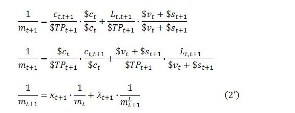
This can be reworked as follows:
In (2′), the reciprocal of the output MELT is expressed as a weighted average of the reciprocals of the input MELT and MELL. The weights κ and λ = 1 – κ (the kappas and lambdas) involve only monetary magnitudes:
It is now possible to apply the same procedure as outlined earlier. For periods 1 and 2, (2′) becomes:
Substituting the expression for 1/m1 into the expression for 1/m2 gives:
For period 3:
Substituting for 1/m2:
A pattern has emerged. For period n:
In words, the reciprocal of the period n MELT is a weighted average of the reciprocals of the unobservable period zero MELT and the MELLs of the n periods. This can be expressed more succinctly as:
The weights represented by the omegas are all products of terms involving kappas and lambdas, and these always take values between zero and one. This means that the reciprocal of the temporal MELT can be approximated as:
This approximation formula will be in error by the unobservable amount:
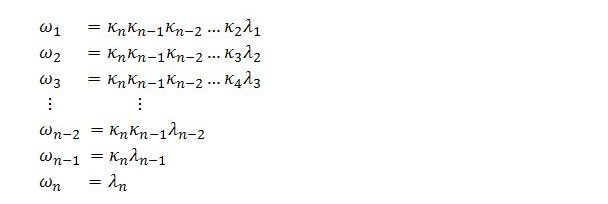
The weights are:
Suppose, for instance, that MELLs and weights are calculated for n = 10 successive periods. Measured in dollars per hour, let’s say that the ten successive MELLs are calculated as 40, 42, 45, 47, 50, 54, 55, 60, 61, 65. It is likely that the unobserved input MELT of period 0 will be no greater than the earliest of the calculated MELLs (or, at the very least, toward the lower end of the values obtained for the MELLs). For simplicity, assume the kappas and lambdas are all 0.5:
Of course, we don’t have the accuracy to justify presenting the answer to this many decimal places. The extra decimals are included because it is still necessary to calculate the reciprocal of this number to arrive at the estimate of the temporal MELT. The error in the estimate of the reciprocal of the MELT is likely to be smaller than:
Taking the appropriate reciprocal, our estimate for the temporal MELT is:
Since the error in the estimate of the MELT’s reciprocal is roughly 0.000024, the true value of the MELT’s reciprocal is probably close to 0.016225515 + 0.000024, implying that the true value for the MELT itself is probably close to:
Calculating MELLs and weights for fewer periods will result in larger error. Conversely, greater accuracy can be achieved by considering more periods. For a given number of periods considered, larger kappas (smaller lambdas) also result in less accuracy.
Once one MELT has been calculated in this manner, the MELTs of later periods can be calculated directly from (1). MELTs of earlier periods can be calculated using a rearrangement of (1):


