Dynamics of Output and Demand in a Growing Economy

by
peterc
My articles My booksMy videos
Follow on:Twitter

An earlier post discussed some of the dynamics of output and demand implicit in the income-expenditure model. Attention was confined to a simplified economy that was stationary other than when adjusting to one-off exogenous changes in demand. The present post considers a continually growing economy in which autonomous demand changes over time. The discussion is kept simple by treating all demand other than private consumption as exogenous. The model can be extended to include additional endogenous demand components – such as investment or job-guarantee spending – but this is left for another time.

 
Behavioral Assumption

As was emphasized in the earlier post, a key behavioral assumption of the income-expenditure model is that, in setting production levels, firms attempt to eliminate unplanned investment, defined as the unanticipated change in inventories. Equivalently, unplanned investment can be defined as excess supply. In response to excess demand or supply, firms are assumed to vary the level of production in an effort to cater to the level of demand. The model presupposes that there is sufficient slack for output to be adjusted to demand in the assumed way.

In the context of a continually growing economy, the elimination of excess demand or supply requires firms not only to react to what has happened in the immediate past (as reflected in any unexpected change in inventories) but also to anticipate how fast demand is likely to grow in the immediate future. This suggests the following decision rule:

This says that firms will adjust actual output (Y) by an amount (ΔY) that is intended to cover the expected change in demand (ΔY_d^e) as well as eliminate part or all (a proportion λ) of unplanned investment (I_u).

If growth is taken to be continuous, with time divisible into tiny increments, the process can be represented in terms of elementary calculus. The above decision rule becomes:

The dots indicate time derivatives. Y dot (= dY/dt) is the instantaneous change in output. Y_d^e dot is the expected change in demand. It equals the expected growth rate of demand (g_d^e) multiplied by the level of total demand: Y_d^e dot = g_d^e Y_d. The level of unplanned investment (I_u) – or excess supply – is the difference between actual output and total demand: I_u = Y – Y_d. Substituting these alternative expressions for Y_d^e dot and I_u into the decision rule and rearranging gives:

 
Expectations

At times it is necessary to specify how expectations are formed. For present purposes, the simplest form of adaptive expectations will do. According to this assumption, firms expect demand in the present to grow at the same rate as it was growing in the recent past:

Here, g_d^e is the expected growth rate of demand at time t and g_dt–θ is the actual growth rate of demand at an earlier time t – θ, where θ is a phase of time.

Adaptive expectations result in systematic errors. When the actual growth of demand is accelerating, so that demand is growing faster now than in the recent past (g_d > g_dt–θ), firms that form expectations in the assumed way will underestimate demand. Conversely, when the growth of demand is decelerating, firms will overestimate demand. Expectations will only turn out to be correct when the growth rate of demand stabilizes for long enough that g_d = g_dt–θ = g_d^e.

This simple form of adaptive expectations implies that, whenever there are errors, expectations are adapted according to the rule:

The difference between g_d^e and g_d is the error in expectations. It is assumed that firms respond by adjusting expectations in the opposite direction to the error. For example, if firms overestimate the growth rate of demand prevailing at time t, the error will be positive. Expectations will be adjusted downwards. This is a special case of a more general rule of adjusting expectations by the amount -β(g_d^e – g_d), where the positive reaction parameter β is set to one.

A different assumption could be made, such as basing expectations on a weighted average of past outcomes, allowing for slower adjustment of expectations in the event of errors, or opting for rational expectations, which would allow for quicker correction of random, unbiased errors, but none of these choices would alter the basic results of the model. One way or another, expectations have to be modeled to give determinate results, but the precise choice does not matter much in the present context as long as the assumed rule is at least somewhat sensible. Accordingly, a simple option is preferred.

 
Growth of Actual Output

Expression (2), which describes the way firms respond to excess demand or supply, implies a growth equation for actual output. This is obtained by dividing both sides of the expression by actual output (Y) and noting that Y dot / Y is the instantaneous growth rate of actual output (g).

If there is excess demand, the fraction Y_d / Y exceeds one and actual output grows faster than expected demand (g > g_d^e). Under excess supply, the reverse is true. Equilibrium requires that demand equal supply (Y_d / Y = 1). In that case, the growth rate of actual output will coincide with the growth rate of expected demand (g = g_d^e).

As has already been noted, expectations can only become correct if the growth of total demand (g_d) first stabilizes. Otherwise, if g_d keeps changing, expectations will also keep changing (with a time delay of θ) and result in variations in the growth rate of actual output.

For equilibrium to persist, firms’ demand expectations would need to become – and then remain – correct (g_d^e = g_d). If this occurred, actual output would grow at the same rate as total demand (g = g_d) until firms made an error in predicting the trajectory of demand. Starting, hypothetically, from a point of equilibrium, any error would cause actual output to deviate from total demand (Y_d / Y would differ from one) and result in diverging growth rates for actual output and total demand.

 
Other Key Assumptions

As has been discussed, the growth equation for actual output given by (5) is predicated on the behavioral assumption that firms, through their production decisions, attempt to eliminate unplanned investment and keep pace with demand. Two other key assumptions of the income-expenditure model are that: (i) there is a positive level of autonomous demand (A > 0); and (ii) there is a positive, and stable, marginal propensity to leak (α > 0) to taxes, saving and imports.

On the basis of these three assumptions, there is a tendency, within the model, for both actual output and demand to converge, at any point in time, toward a particular (but, in a growth context, evolving) level of output (Y*) at which supply would equal demand.

The characterization of this equilibrium level of output will depend on what is assumed about demand. As always, total demand can be considered as the sum of two parts: induced demand and autonomous demand. Here, all demand other than net induced consumption is assumed to be autonomous. This makes induced demand (1 – α)Y. Autonomous demand is A. Therefore:

 
Equilibrium Output

With the determinants of actual output and total demand specified, the level of output (Y*) to which supply and demand converge can be established. With actual output equal to total demand, Y and Y_d can be replaced with Y* in (6):

Solving for Y* gives:

Output level Y* is a particular multiple (equal to 1_{/α) of autonomous demand. It is a notional level of output (changing over time) that the economy does not necessarily reach. Its relevance hinges on it being an ‘attractor’ for both actual output and total demand. In the income-expenditure model, Y* does in fact play the role of an attractor under most circumstances. A way to verify this point is presented later.}

 
Growth of Equilibrium Output

The growth rate of Y* can be obtained from (6′). The first step is to differentiate with respect to time:

All terms involving Y* dot can be collected to the left-hand side:

Dividing through by αY* will convert the left-hand side to a growth rate (Y* dot / Y*). Multiplying A dot by A / A will also enable this derivative to be converted to a growth rate:

Rewriting the expression in terms of growth rates and noting that A / α = Y* gives:

Under present assumptions, the growth rate of Y* simply follows the behavior of autonomous demand (g* = g_A), which is taken as exogenously given.

 
Growth of Total Demand

The growth behavior of total demand is implicit in (6). Following the same procedure as in the previous section, the expression can be differentiated with respect to time:

Dividing through by Y_d and multiplying Y dot and A dot by Y / Y and A / A, respectively, gives:

Expressed in terms of growth rates:

Here, g_d, g and g_A are the growth rates of total demand, actual output and autonomous demand, respectively. The growth rate of total demand is basically a weighted average of the growth rates of actual output (g) and autonomous demand (g_A). The first term on the right-hand side describes endogenous demand growth. The second term describes autonomous demand growth.

Substituting for g, using (5), and rearranging yields the following expression for the growth rate of total demand:

Terms 1 and 2 can be considered briefly in turn. If there is excess demand, Y / Y_d is less than one and term 1 will be greater than (1 – α) g_d^e. As Y / Y_d increases toward one, the term approaches (1 – α) g_d^e. If Y / Y_d actually equals one, the term will equal (1 – α) g_d^e. Now, it has already been mentioned, in relation to (5), that when Y / Y_d equals one, the growth rate of actual output equals both the expected growth rate of demand (g = g_d^e) and, by (8), the growth rate of autonomous demand (g = g_A = g*). So the tendency of term 1 is to approach (1 – α) g*.

Turning to term 2, in equilibrium A_{/Yd equals α. This is clear because, from (7), the equilibrium level of income is Y = Yd = Y* = A/α, implying A/Y = A/Yd = α. When there is excess demand, both Y and Yd are less than Y*, implying Yd < A/α or, upon rearrangement, A/Yd > α. So term 2 exceeds αgA when there is excess demand but tends toward αgA as A/Y shrinks toward α. In equilibrium, term 2 equals αgA. And since gA is the equilibrium growth rate, term 2 tends toward αg*.}

Considering the right-hand side of (10) as a whole, the growth rate of demand (g_d) tends to approach (1 – α)g* + αg* = g*.

 
Dynamic Stability

The discussion so far has highlighted certain characteristics of ‘equilibrium’ – or what is often referred to as ‘steady state’ – growth. In a nutshell, a steady state would require actual output continually to equal total demand (Y = Y_d = Y* = A / α). Under these circumstances, autonomous demand would be a stable fraction (α) of actual output and total demand (A / Y = A / Y_d = α). In terms of growth rates, all key variables would be growing at the same rate (g = g_d^e = g_d = g_A = g*).

Of course, it is one thing to identify features of steady-state growth. It is another to establish whether the system has a tendency to move toward such a state. Basically, the question is this: if the exogenously given growth rate of autonomous demand is held constant for long enough, will the assumed behavior of firms and households tend to push the economy toward a situation in which actual output and total demand converge on output level Y* with all key variables growing at the same rate as autonomous demand?

It should be stressed that this is an exercise more in logic than empirical reality. There is no suggestion that autonomous demand would in fact grow at a constant rate for any significant length of time or that a real-world economy could ever attain a steady state. The purpose of the exercise is to establish the results and tendencies that follow, logically, from the stated assumptions of the model.

To consider the issue of dynamic stability, let:

Variables y and z, both ratios, are measures of excess demand. Variable y is greater than, equal to, or less than one depending on whether demand is greater than, equal to, or less than output. When Y = Y_d = Y*, y = 1.

Variable z, the share of autonomous demand in income, is an alternative indicator of excess demand. It has already been observed that when demand and supply are both at the level Y*, z = α. If, starting from a steady state, autonomous demand subsequently grows at a different rate than output, there will be excess demand or supply, with z diverging from α. Under excess demand, z > α; under excess supply, z < α.

It follows from the definitions of y and z that the share of autonomous demand in total demand (A / Y_d) is z / y. As with z, this share is greater than, equal to, or less than α depending on whether there is excess demand, equilibrium, or excess supply.

Most of our focus can be on variable y (= Y_d / Y). Dynamic stability requires y to tend toward one and, if it gets there, to remain at one unless there is an exogenous change in either the growth rate of autonomous demand (g_A) or the marginal propensity to leak (α). Clearly, whether y will behave in the required way will depend on the growth behavior of total demand (Y_d) and actual output (Y). This can be made explicit by differentiating y with respect to time (applying the quotient rule):

The fractions in brackets on the far right are growth rates and Y_d / Y is variable y. Modifying the expression accordingly gives:

This is a differential equation. It relates the instantaneous change in y (y dot = dy/dt) to the growth rates of demand and output (g_d and g) as well as to y itself.

For a steady state to persist, it is not enough that y = 1 at a given moment. It is also necessary for y to remain unchanged (y dot = 0). As (12) spells out, this can only occur if demand and output happen to grow at the same rate (g_d = g = g*).

Equation (12) is missing details that are needed to assess stability. One way to fill in these details is to express the equations for g_d and g in terms of y and substitute the resulting expressions into (12). An alternative way, which turns out to be a bit simpler, is to substitute an equation for g into an equivalent expression for y dot, making use of the definition of z. The first step is to differentiate z ( = A / Y) with respect to time to obtain:

It can then be observed that

Since both 1 and α are constants, it follows that y and z both change at the same rate:

This means that the expression for z dot in (13) can be substituted into the right-hand side of (12) to obtain:

To eliminate z, it can be noted from rearrangement of (14) that z = y + α – 1. Upon substituting for z, (12) becomes:

Since (12) and (12′) are equivalent expressions, either can be used to check stability.

It is still necessary to substitute an expression for g in (12′). Writing (5) in terms of y gives the required expression:

Substituting this into (12′) gives:

Formulated in terms of (12”), the question of dynamic stability comes down to how y dot responds to a small change in y. Starting from a situation in which y = 1 and y dot = 0, it is necessary that changes in y away from 1 set in motion forces that tend to cause y to move back toward 1. In considering this question, expectations will be taken as given. At time t they are already formed, based on what happened at time t – θ. And if a steady state has persisted at least for length of time θ, the expected growth rate of demand will equal the other growth rates under consideration. The other elements in (12”) are either parameters (α, λ) or an exogenous variable (g_A) and so can also be taken as given. Accordingly, we take the derivative of y dot with respect to y. Dynamic stability requires that the derivative be negative when evaluated at the critical point y = 1, y dot = 0.

In undertaking this exercise, it is important to mention that equation (12”) is nonlinear in y because of a y-squared term (if the expression is expanded out). This means that taking the derivative with respect to y serves only as a test of ‘local stability’ as opposed to ‘global stability’. Basically, the derivative represents the best linear approximation to the behavior of y near the point y = 1.

Taking the relevant derivative (applying the product rule) gives:

Evaluating the derivative where y = 1 and g_d^e = g_A = g* reduces the expression to:

The derivative is negative provided:

Therefore, the modeled behavior is locally stable provided the growth rate of autonomous demand (g_A = g*) exceeds -λ, where λ is the positive reaction parameter that indicates the intensity of firms’ response to unanticipated changes in inventories. For positive growth regimes, the model always exhibits local stability.

 
Description of the Model’s Growth Behavior

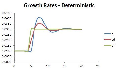
Provided the condition for dynamic stability holds (g* > -λ), and y stays quite close to 1, the behavioral assumptions ensure a tendency for actual output and total demand to converge on Y*. Conceptually, the growth process depicted in the model can be described as follows. Starting from a steady state, an exogenous increase in the growth rate of autonomous demand (g_A) creates a situation in which actual output and, to a lesser extent, total demand temporarily grow less rapidly than Y*. This results in excess demand (y > 1), a delayed upward revision of expectations (since g_d > g_dt–θ), and an acceleration of output growth (g) that brings with it further endogenous acceleration of demand growth (g_d). So long as g remains below g_A, it also remains below g_d. At this stage, y is still rising further above one.

At a certain point, g catches up to g_d. This occurs at the same time as g catches up to g_A. It then overtakes both g_d and g_A. The deviation of g above g_A is greater than g_d‘s deviation. This is partly because endogenous demand growth accounts for only a fraction of total demand growth (which is a weighted average of endogenous and exogenous growth) and partly because leakage to taxes, saving and imports occurs throughout the process.

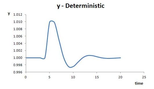
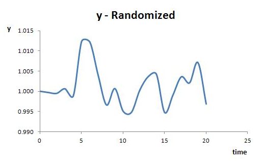
In the convergence of y toward 1, there can be some oscillation (fluctuation) around the critical point. This is due to the lag in firms’ response to excess demand and supply, including in the adjustment of expectations. If the growth rate of autonomous demand (g_A) is held constant throughout the adjustment process, the oscillation is damped (declining in amplitude). This is illustrated in the first diagram below. In the second diagram, random variations in g_A cause more sporadic behavior. In both diagrams, the growth rate of autonomous demand is exogenously increased from 0.01 to 0.03 at time t = 5, though with random variation around these levels in the second diagram.

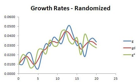
The next two diagrams illustrate the convergence of growth rates. Once again, the growth rate of autonomous demand is exogenously increased from 0.01 to 0.03 at time t = 5. In the first diagram, the process is entirely deterministic. In the second diagram, the growth rate of autonomous demand is subjected to random disturbance.

The way in which g interacts with g_d and g_A can be verified working from the expression for g_d in (9). Subtracting g from both sides of the expression gives:

This can be rewritten

In the first fraction on the right-hand side, the difference between total demand Y_d and induced demand (1 – α)Y is simply autonomous demand A. Modifying the expression accordingly gives:

If g is less than g_A, the right-hand side is positive. Since the left-hand side must then also be positive, g will clearly be less than g_d. Conversely, when g is greater than g_A, it must also be greater than g_d. This confirms that g deviates further from g_A in both directions than g_d deviates. The expression also shows that the growth rates of actual output and total demand coincide when equal to the growth rate of autonomous demand (g = g_d = g_A).