Introductory Macroeconomics with a Job Guarantee

by
peterc
My articles My booksMy videos
Follow on:Twitter

In some earlier posts, a job guarantee is added to an otherwise condensed income-expenditure model. This enables comparisons of steady states under different scenarios akin to the typical exercises conducted in introductory macroeconomics courses. What follows is a summary of the model, bringing together aspects that are dealt with in greater depth – but disparately – elsewhere on the blog, along with brief indications of how the model can be extended to include simple dynamics and short-run price behavior. Links to fuller explanations of various concepts are provided along the way.

 
Simplifying assumptions

The model composes the economy into sector b and sector j. Sector j is the job guarantee sector. Its operations are confined to the activity of workers employed in the job guarantee program. Sector b is the broader economy, which includes the public sector other than job guarantee activity, the domestic private sector and the external sector. It is supposed that plant, equipment and materials used in the job guarantee program, as well as public administration of the program, are supplied by the broader economy. It is assumed, as in earlier posts, that inputs into job guarantee production are purchased from the domestic economy. The final section notes briefly how the model can be modified to allow for imported inputs.

The simple short-run model considered here has the following features:

1. Productive capacity is fixed.

2. The level of total employment is exogenously given. The sectoral composition of employment varies endogenously.

3. Productivity is higher in sector b than in sector j. Productivity within each sector is taken as given. This implies that average productivity for the economy as a whole varies endogenously and procyclically as workers switch between the two sectors.

4. Induced household consumption expenditure (considered net of endogenous taxes and endogenous imports) and the government’s job guarantee spending are endogenous. All other categories of spending are exogenous. They are considered net of exogenous taxes and exogenous imports and simply grouped together as autonomous demand. These expenditures include autonomous household consumption expenditure, private investment, government spending other than on the job guarantee, and exports.

5. A constant fraction of an increment in income drains to taxes, saving and imports.

 
Basic model

The model is depicted in steady-state condition (1) and behavioral equations (2) to (4):

Steady state condition (1) requires total output Y to be adjusted to total demand Y_d. Total demand is the sum of induced net consumption C_I, job guarantee spending G_j and autonomous demand A, as shown in (2). According to (3), induced consumption is positively related to total income, where α is the constant marginal propensity to leak. According to (4), job guarantee spending is inversely related to total income.

Examining (4) a little more closely, the government’s spending on the job guarantee is interpreted as a fraction q of the ‘output gap’, here defined to be the difference between maximum possible output ρ_bL and actual output Y. Maximum possible output is the output that would be produced if all employment L could be located in sector b operating with productivity ρ_b. Due to the requirements of price stability, this level of output will not be tolerated by policymakers. To the extent that some employment is located in sector j, actual output will fall short of the maximum possible, resulting in the output gap ρ_bL – Y.

The fraction q is constant under present assumptions. From (4),

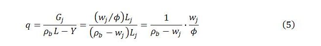where w_j is the exogenously given job guarantee wage, taken to define sector j productivity, and ϕ is the wage share in job guarantee spending, assumed for simplicity to be constant. The logic underpinning (5) is explained in part 2 of a recent series on the job guarantee in the subsection on job guarantee spending.

Substituting (3) and (4) into (2) gives the demand function:

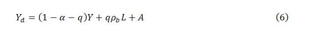Substituting this expression into (1) and solving for Y gives the steady-state level of total output:

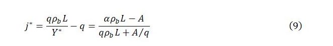
It is convenient to define j as the ratio of job guarantee spending to total income. Dividing both sides of (4) by Y gives

This says that j varies inversely with total income. In a steady state, j stabilizes:

In general, the sectoral levels of output are endogenously determined proportions of total output:

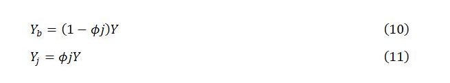
In a steady state,

Expressions for Y_b* and Y_j* involving only parameters and exogenous variables can be obtained by substituting for j* and Y* in (10′) and (11′). These and other aspects of the steady state are outlined in the first section of an earlier post.

The model in this simple form can be represented in terms of the familiar Keynesian cross diagram, as explained in part 2 of the job guarantee series linked to above.

As also explained in an earlier post, simple dynamics can be introduced into the model by positing that sector b output changes in proportion to excess demand. This, in turn, implies particular dynamics for sector j output and total output. It can be shown (see here) that, for given values of the parameters and exogenous variables, the system always tends toward the steady state.

A short-run relationship between the price level and total output can be introduced by assuming markup or normal pricing but allowing for a demand influence over the business cycle. Letting P₀ denote a purely supply-determined price level that would prevail in the absence of excess demand or excess supply pressures and supposing that deviations from this price level reflect demand conditions, it can be specified for instance that

where R is the fraction of total employment located in sector j (the buffer employment ratio), R_n is the buffer employment ratio that occurs when excess demand pressures are absent (assumed to correspond to normal output Y_n), and β is a positive parameter measuring the sensitivity of prices to fluctuations in demand. Price equation (12), which reflects an inverse relationship between the price level and the buffer employment ratio, implies a corresponding direct relationship between the price level and total output. For small values of β, the price level is very stable over a fairly wide range of output near Y_n but escalates as the economy nears maximum possible output. The supply-determined P₀ will be susceptible to influence through the government’s role as price setter in, at minimum, the establishment of the job guarantee wage. Fluctuations in demand will be moderated, in part, by the automatic stabilizing properties of the job guarantee along with other automatic stabilizers and any countercyclical discretionary actions by government. A fuller discussion can be found here.

 
Allowing for imported inputs in sector j production

If the government imported some of the equipment and materials used in job guarantee production, not all job guarantee spending would contribute to total demand. The model can be modified to allow for this. Letting m_j denote the fraction of job guarantee spending going to imports, and treating this fraction as constant, equation (2) of the basic model becomes

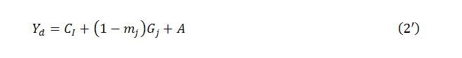
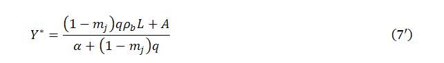
If ϕ, the wage share in job guarantee spending, were permitted to vary, it would be necessary to subtract (1 – ϕ)m_jG_j from G_j rather than subtracting m_jG_j as in (2′). But so long as ϕ is assumed constant, as it is here and in earlier treatments, the modification given by (2′) suffices. This modifies the demand function to

implying steady-state total output of

To make the most of the stabilizing properties of the job guarantee, it would probably make sense for government to avoid or at least minimize the importing of sector j inputs. With this in mind, it seems preferable to skip the slight complication of imported inputs and assume all job guarantee spending is on the domestic economy.