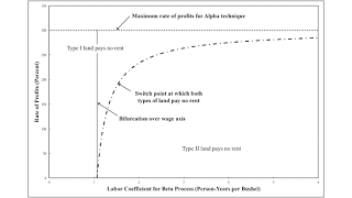
Figure 1: A Bifurcation Diagram1.0 Introduction I have been looking at how bifurcation analysis can be applied to the choice of technique in models in which all capital is circulating capital. In my sense, a bifurcation occurs when a switch point appears or disappears off the wage frontier. A question arises for me about how to apply or visualize bifurcations in models with land, fixed capital, and so on. This post starts to investigate this question by looking at a numerical example of a overly simple model with land and extensive rent. 2.0 Parameters and Assumptions for the Model Table 1 specifies the technology for this example. One parameter, the labor coefficient a0β, is left free. Managers of firms know of two processes for producing corn from inputs of labor, (a type of)
Topics:
Robert Vienneau considers the following as important: Example in Mathematical Economics, Joint Production
This could be interesting, too:
Robert Vienneau writes Austrian Capital Theory And Triple-Switching In The Corn-Tractor Model
Robert Vienneau writes Double Fluke Cases For Triple-Switching In The Corn-Tractor Model
Robert Vienneau writes The Emergence of Triple Switching and the Rarity of Reswitching Explained
Robert Vienneau writes Recap For A Triple -Switching Example

|
| Figure 1: A Bifurcation Diagram |
I have been looking at how bifurcation analysis can be applied to the choice of technique in models in which all capital is circulating capital. In my sense, a bifurcation occurs when a switch point appears or disappears off the wage frontier. A question arises for me about how to apply or visualize bifurcations in models with land, fixed capital, and so on.
This post starts to investigate this question by looking at a numerical example of a overly simple model with land and extensive rent.
2.0 Parameters and Assumptions for the ModelTable 1 specifies the technology for this example. One parameter, the labor coefficient a0β, is left free. Managers of firms know of two processes for producing corn from inputs of labor, (a type of) land, and seed corn. Each process is defined in terms of coefficients of production. All processes exhibit constant returns to scale; require a year to complete; and totally use up, in producing their output, the capital good required as input. Land, of the specified type, exits the production process as good as it was at the start of the year.
| Input | Corn Industry | ||
| Alpha | Beta | ||
| Labor | a0α = 1 Person-Yr. | a0β Person-Yr. | |
| Land | bα = 10 Acres of Type I | bβ = 20 Acres of Type II | |
| Corn | aα = (1/4) Bushels | aβ = (1/5) Bushels | |
Each type of land is in fixed supply:
- LI = 100 Acres of Type I land exist.
- LII = 100 Acres of Type II land exist.
The assumptions so far impose some limits on the quantity of net output that can be produced. If only Type I land is seeded, and that land is fully used, net output consists of:
(1 - aα) LI/bα = (15/2) bushels
Likewise, if only Type II land is seeded, net output consists of 4 bushels. If net output exceeds (15/2) bushels (that is, the maximum of 15/2 and 4 bushels), both types of land will need to be seeded. If net output is less than (23/2) bushels (that is, the sum of 15/2 and 4 bushels), at least one type of land will not be fully used. Accordingly, assume:
(15/2) bushels < y < (23/2) bushels
where y is net output. Under these assumptions, one type of land is in excess supply and pays no rent.
I consider prices of production to determine rent and to find out which land is free. Since net output is taken here as a constant, no matter how much a0β may fall, I am assuming increased productivity (per worker) is taken in the form of decreased employment.
3.0 Price EquationsI take corn to be numeraire, and I assume rent and wages are paid out of the surplus at the end of the period. Prices of production must satisfy the following system of equations:
(1/4)(1 + r) + 10 ρI + w = 1
(1/5)(1 + r) + 20 ρII + a0βw = 1
where r, w, ρI, and ρII are the rate of profits, the wage, the rent on Type I land, and the rent of Type II land. All four of these distribution variables are assumed to be non-negative. The condition that at least one type of land pays a rent of zero is expressed by a third equation:
ρI ρII = 04.0 The Choice of Technique
I consider three solutions of the price equation, each for a different parameter value of a0β.
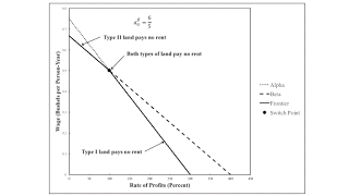
4.1 First ExampleFirst, suppose a0β is (6/5) person-years per bushel. Each process yields a wage curve, under the assumption that the corresponding type of land pays no rent. Figure 1 graphs both wage curves. A simple generalization of this model would be to multiple produced commodities, with land only used in one industry. Each process in that industry would be associated with a technique, and the associated wage curve could be of any convexity, with the convexity possibly varying throughout its extent.

|
| Figure 2: Each Type of Land Sometimes Pays Rent |
In this example, in which both types of land must be used to produce the given net output, the relevant frontier is the inner frontier, shown as a solid black line in the figure. This, too, does not generalize to a multi-commodity model with more types of land. In that case, one would work from the outer frontier inward until the successive types of land could produce, at least, the given net output. This order might depend on whether the wage or the rate of profits was taken as given. Or perhaps some other theory of distribution could be analyzed.
Anyways, the type of land associated with the technique on the inner frontier, in this example, pays no rent. For low rates of profits or high wages, Type II land pays no rent. For high rates of profits or low wages, Type I land pays no rent. At the switch point, both types of land pay no rent. If the wage were given, rent on the type of land associated with the process further from the origin would come out of the super profits that would otherwise be earned on that process. If the rate of profits were given, one might see a conflict between workers and landlords. This analysis is a matter of competitive markets, inasmuch as capitalists can move their investments among industries and processes.
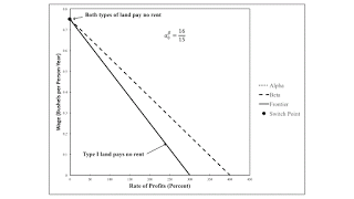
4.2 Bifurcation Over Wage AxisI next consider a parameter value for a0β of (16/15) person-years per bushel. As shown in Figure 2, this is a case of a bifurcation over the wage axis. You cannot see the wage curve for the Alpha technique in the figure because it is always on the inner frontier. For any distribution of the surplus, Type I land pays no rent. If the rate of profits is zero, Type II land also pays no rent. For any positive rate of profits, landlords obtain a rent on Type II rent.

|
| Figure 3: A Bifurcation Over the Wage Axis |
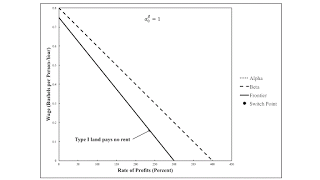
For a final case, let a0β be one person-years per bushel. The wage curve for the Alpha technique has now rotated downwards counter clockwise so far that it never intersects the wage curve for the Beta technique. Whatever the distribution, Type I land pays no rent, and owners of Type II land receive a rent.

|
| Figure 4: Wage Curves Never Intersect |
So this simple example can be illustrated with a bifurcation diagram, as seen at the top of this post. The rate of profits for the switch point is"
rswitch = (15 a0β - 16)/(5 a0β - 4)
This function asymptotically approaches the maximum rate of profits for the Alpha technique as a0β increases without bound. The wage curve for Alpha continues to become steeper and steeper. I suppose wage for the switch point approaches the wage on the wage curve for the Beta technique when the rate of profits is 300 percent.
One can also solve for the rents. When the rent on Type I land is non-negative, it is:
ρI = [(15 a0β - 16) + (4 - 5 a0β)r]/(200 5 a0β)
When the rent on Type II land is non-negative, it is:
ρII = [(16 - 15 a0β) + (5 a0β - 4)]/4005.0 Conclusions
I am partly interested in bifurcation analysis because one can draw neat graphs to visualize the economics. For the numerical example, I would like to be able to draw three-dimensional diagrams. Imagine an axis coming out of the page for the bifurcation digram at the top of this post. I then could have a surface where the rent on one of the types of land is graphed against the rate of profits and the coefficient of production being varied parametrically.
It seems like all four of the normal forms for bifurcations of co-dimension one that I have defined may arise in examples of extensive rent. These are a bifurcation over the wage axis, a bifurcation over the axis for the rate of profits, a three-technique bifurcation, and a restitching bifurcation. They will not necessarily be on the outer frontier, however.
I think another type of bifurcation may be possible. Suppose productivity increases because coefficients of production decreases for land inputs or inputs of capital goods. Given net output, could such an increase in productivity result in some type of land that formerly paid rent (for some range of the rate of profits) becoming rent-free? Could all types of land become non-scarce? How would this sort of bifurcation look on an appropriate bifurcation diagram? Would the distinction between the order of rentability and efficiency be reflected in bifurcation analysis? Can I draw a bifurcation diagram with a discontinuity?
 Heterodox
