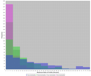
Figure 1: Blowup of Distribution of Maximum Rate of Profits This post extends the results from my last post. I think of the results presented here as providing information about the implementation of my simulation. I do not claim any implications about actually existing economies. I did not have any definite anticipations about what I would see. I suppose it could be of interest to regenerate these results where coefficients of production are randomly generated from some non-uniform distribution. I continue to use a capability to generate a random economy, where such an economy is characterized by a single technique. A technique is specified by a row vector of labor coefficients and a corresponding square Leontief input-output matrix. The labor coefficients are randomly generated from
Topics:
Robert Vienneau considers the following as important: Example in Mathematical Economics
This could be interesting, too:
Robert Vienneau writes Austrian Capital Theory And Triple-Switching In The Corn-Tractor Model
Robert Vienneau writes Double Fluke Cases For Triple-Switching In The Corn-Tractor Model
Robert Vienneau writes The Emergence of Triple Switching and the Rarity of Reswitching Explained
Robert Vienneau writes Recap For A Triple -Switching Example

|
| Figure 1: Blowup of Distribution of Maximum Rate of Profits |
This post extends the results from my last post. I think of the results presented here as providing information about the implementation of my simulation. I do not claim any implications about actually existing economies. I did not have any definite anticipations about what I would see. I suppose it could be of interest to regenerate these results where coefficients of production are randomly generated from some non-uniform distribution.
I continue to use a capability to generate a random economy, where such an economy is characterized by a single technique. A technique is specified by a row vector of labor coefficients and a corresponding square Leontief input-output matrix. The labor coefficients are randomly generated from a uniform distribution on (0.0, 1.0]. Each coefficient in the Leontief input-output matrix is randomly generated from a uniform distribution on [0.0, 1.0). The random number generator is as provided by the class java.util.Random, in the Java programming language. I am running Java version 1.8.
Each random economy is tested for viability. Non-viable economies are discarded. Table 1 shows how many economies needed to be generated, given the number of produced commodities, to end up with a sample size of 300 viable economies. The maximum rate of profits is calculated for each viable economy. The maximum rate of profits occurs when the wage is zero, and the workers live on air. Thus, labor coefficients do not matter for the calculation of the maximum rate of profits.
| Seed for Random Generator | Number of Commodities |
Number of Economies |
| 368,424,234 | 2 | 610 |
| 345,657 | 3 | 6,124 |
| 4,566,843 | 4 | 826,471 |
| 547,527 | 5 | > 231 - 1 |
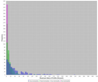
I looked at the distribution of the maximum rate of profits, calculated as a percentage, in several ways. Figure 2 presents four histograms, superimposed on one another. Figure 1 expands the left tails of these histograms. I suppose Figure 2 is somewhat easier to make sense of than Figure 1, when you click on the image. Maybe the statistics in Tables 2 and 3 are clearer. One can see, for example, in random economies in which two commodities are produced, the mean of the maximum rate of profits is 43.9%. The minimum, in these 300 random economies, of the maximum rate of profits is about 0.03% and the maximum is 318%. If I wanted to be more thorough, I would have to review how skewness and kurtosis are calculated by default in the Java class org.apache.commons.math3.stat.descriptive.DescriptiveStatistics. The coefficient of variation is the ratio of the standard deviation to the mean. The nonparametric analogy, reported in the last row in Table 3, is the ratio of the Inter-Quartile Range to the median. Anyways, the distribution of the maximum rate of profits, in random viable economies generated by the simulation, is non-Gaussian and highly skewed, with a tail extending to the right.

|
| Figure 2: Distribution of Maximum Rate of Profits |
| Number of Produced Commodities | |||||
| Two | Three | Four | Five | ||
| Sample Size | 300 | 300 | 300 | 300 | |
| Mean | 43.9 | 15.7 | 8.28 | 4.95 | |
| Std. Dev. | 50.2 | 19.3 | 7.53 | 5.90 | |
| Skewness | 2.10 | 3.89 | 1.22 | 2.63 | |
| Kurtosis | 5.14 | 22.2 | 0.882 | 9.64 | |
| Coef. of Var. | 0.875 | 0.811 | 1.10 | 0.839 | |
| Number of Produced Commodities | |||||
| Two | Three | Four | Five | ||
| Minimum | 0.0327 | 0.113 | 0.0107 | 0.00405 | |
| 1st Quartile | 9.35 | 4.51 | 2.52 | 1.17 | |
| Median | 25.3 | 9.72 | 5.70 | 2.99 | |
| 3rd Quartile | 57.3 | 19.9 | 11.3 | 6.27 | |
| Maximum | 318 | 168 | 36.2 | 44.2 | |
| IQR/Median | 1.90 | 1.58 | 1.54 | 1.70 | |
With the simulation, the maximum rate of profits tends to be smaller, the more commodities are produced. I wish I could extend these results to a lot more produced commodities. National Income and Product Accounts (NIPAs), at the grossest level of aggregation have on the order of 100 produced commodities. Even if results with the assumption of an arbitrary probability distribution for coefficients of production could be directly applied empirically, one would like confirmation that trends seen with a very small number of produced commodities continue.
 Heterodox
