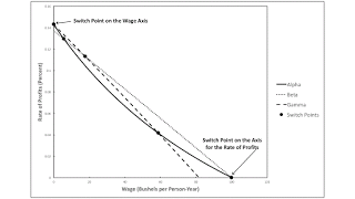
Figure 1: Fluke Switch Points on Each Axis1.0 Introduction I have developed an approach for finding examples in which either two fluke switch points exist on the wage frontier or a switch point is a fluke in more than one way. This post presents a numerical example with two fluke switch points on the frontier. Not all examples generated by this approach are necessarily interesting, although I find the approach of interest. I don't think the example in this approach is all that fascinating. I had thought that examples of real Wicksell effects of zero were somewhat interesting, but I have received disagreement. Anyways, what I have been doing is drawing bifurcation diagrams for examples in which coefficients of production vary. The bifurcation diagram partitions a parameter space into
Topics:
Robert Vienneau considers the following as important: Example in Mathematical Economics, Sraffa Effects
This could be interesting, too:
Robert Vienneau writes Austrian Capital Theory And Triple-Switching In The Corn-Tractor Model
Robert Vienneau writes Double Fluke Cases For Triple-Switching In The Corn-Tractor Model
Robert Vienneau writes The Emergence of Triple Switching and the Rarity of Reswitching Explained
Robert Vienneau writes Recap For A Triple -Switching Example

|
| Figure 1: Fluke Switch Points on Each Axis |
I have developed an approach for finding examples in which either two fluke switch points exist on the wage frontier or a switch point is a fluke in more than one way. This post presents a numerical example with two fluke switch points on the frontier. Not all examples generated by this approach are necessarily interesting, although I find the approach of interest. I don't think the example in this approach is all that fascinating. I had thought that examples of real Wicksell effects of zero were somewhat interesting, but I have received disagreement.
Anyways, what I have been doing is drawing bifurcation diagrams for examples in which coefficients of production vary. The bifurcation diagram partitions a parameter space into regions in which the sequence of switch points does not vary, even though their specific locations on the wage frontier may. The loci dividing regions with topologically equivalent wage frontiers specify fluke cases. A point in the parameter space in which more than one such loci intersect specifies an example which is a fluke in more than one way.
2.0 TechnologyThe example is a numerical instantiation of the Samuelson-Garegnani model. A single consumption good, corn is produced from inputs of corn and one of three capital goods. Table 1 lists the coefficients of production for production processes for producing corn. Each production process in this example requires a year to complete and exhibits Constant Returns to Scale. A column in Table 1 lists the physical inputs for that process required per unit corn produced at the end of the year. Workers labor over the course of the year, and the inputs of the capital good are totally used up in the process. Managers of firms also know of a process for producing each capital good (Table 2). For a given capital good, the process for producing it requires inputs of labor and the services of that capital good.
| Input | Corn Industry | ||
| Alpha | Beta | Gamma | |
| Labor | 1 | 3.69174 | 3.33574 |
| Iron | 3 | 0 | 1 |
| Copper | 0 | 0.92850 | 0 |
| Uranium | 0 | 0 | 1.79455 |
| Corn | 0 | 0 | 0 |
| Input | Industry | ||
| Iron | Copper | Uranium | |
| Labor | 1 | 1.94290 | 0.917647 |
| Iron | 0.5 | 0 | 1 |
| Copper | 0 | 0.5 | 0 |
| Uranium | 0 | 0 | 0.550588 |
| Corn | 0 | 0 | 0 |
Any one of three techniques can be adopted to sustainably produce corn. The Alpha technique consists of the iron-producing process and the corresponding, labelled process for producing corn. The Beta technique consists of the copper-producing process and corresponding for producing corn. And similarly for the Gamma technique.
3.0 Prices and the Wage FrontierFor each technique, a system of two equations arises. I take corn as the numeraire and assume that labor is paid out of the surplus at the end of the year. The equations show the same rate of profits being earned for both processes comprising a technique. Given an externally specified rate of profits, the equations are a linear system. They can be solved for the wage and the price of the capital good, as functions of the rate of profits. For the wage, this function is known as the wage curve. All three wage curves, one for each technique, are graphed in Figure 1 above.
The wage frontier consists of the outer envelope of all wage curves. The curve(s) on the frontier at a given rate of profits correspond(s) to the cost-minimizing technique(s) at that rate of profits. The Gamma technique is cost-minimizing at low rates of profits, and the Beta technique is cost-minimizing at high rates of profits. These two techniques are tied - that is, both cost-minimizing - at the switch point dividing these two regions of the rate of profits.
The Alpha technique is only cost-minimizing at the switch points on the wage axis and on the axis for the rate of profits. And, it is tied, with the Gamma and Beta techniques, respectively, at these switch points. A switch point appearing on the wage axis or the axis for the rate of profits is a fluke case. So both switch points with the Alpha technique are flukes. Having Alpha participate in two fluke switch points is even more of a fluke case. For what it is worth, the fluke switch point on the axis for the rate of profits exhibits capital-reversing.
 Heterodox
