Figure 1: Bifurcation Diagram1.0 Introduction I have been exploring the variation in the number and "perversity" of switch points in a model of prices of production. I conjecture that generic changes in the number of switch points with variations in model parameters can be classified into a few types of bifurcations. (This conjecture needs a more precise statement.) This post fills a lacuna in this conjecture. I give an example of a case that I have not previously illustrated. 2.0 Technology Consider the technology illustrated in Table 1. The managers of firms know of four processes of production. And these processes exhibit Constant Returns to Scale. The column for the iron industry specifies the inputs needed to produce a ton of iron. In this post, I consider how variations in the
Topics:
Robert Vienneau considers the following as important: Example in Mathematical Economics, Labor Markets, Sraffa Effects
This could be interesting, too:
Robert Vienneau writes Austrian Capital Theory And Triple-Switching In The Corn-Tractor Model
Robert Vienneau writes Double Fluke Cases For Triple-Switching In The Corn-Tractor Model
Robert Vienneau writes The Emergence of Triple Switching and the Rarity of Reswitching Explained
Robert Vienneau writes Recap For A Triple -Switching Example

|
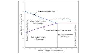
| Figure 1: Bifurcation Diagram |
I have been exploring the variation in the number and "perversity" of switch points in a model of prices of production. I conjecture that generic changes in the number of switch points with variations in model parameters can be classified into a few types of bifurcations. (This conjecture needs a more precise statement.) This post fills a lacuna in this conjecture. I give an example of a case that I have not previously illustrated.
2.0 TechnologyConsider the technology illustrated in Table 1. The managers of firms know of four processes of production. And these processes exhibit Constant Returns to Scale. The column for the iron industry specifies the inputs needed to produce a ton of iron. In this post, I consider how variations in the parameter e affect the number of switch points. The column for the copper industry likewise specifies the inputs needed to produce a ton of copper. Two processes are known for producing corn, and their coefficients of production are specified in the last two columns in the table. Each process is assumed to require a year to complete and uses up all of its commodity inputs.
| Input | Industry | |||
| Iron | Copper | Corn | ||
| Alpha | Beta | |||
| Labor | e | 3/2 | 1 | 3/2 |
| Iron | 1/4 | 0 | 1/4 | 0 |
| Copper | 0 | 1/5 | 0 | 1/5 |
| Corn | 0 | 0 | 0 | 0 |
This technology presents a problem of the choice of technique. The Alpha technique consists of the iron-producing process and the corn-producing process labeled Alpha. Similarly, the Beta technique consists of the copper-producing process and the corn-producing process labeled Beta.
The choice of technique is based on cost-minimization. Consider prices of production, which are stationary prices that allow the economy to be reproduced. A wage curve, showing a tradeoff between wages and the rate of profits, is associated with each technique. In drawing such a curve, I assume that a bushel corn is the numeraire and that labor is advanced. Hence, wages are paid out of the surplus product at the end of the year. The chosen technique, for, say, a given wage, maximizes the rate of profits. The wage curve for the cost-minizing technique at the given wage lies on the outer frontier formed from all wage curves.
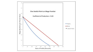
3.0 A Result of Technical ProgressFor a high value of the parameter e, the Beta technique minimizes costs, for all feasible wages and rates of profits. Figure 2 illustrates wage curves when e is equal to 21/8. For any wage below the maximum, the Beta technique is cost minimizing. But at a rate of profits of zero, a switch point arises. Both techniques are cost-minimizing.

|
| Figure 2: A Switch Point on the Wage Axis |
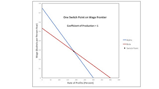
Suppose technical progress further decreases the person-years needed as input for each ton iron produced. Figure 3 illustrates wage curves when e has fallen to one. For low wages, the Beta technique is cost-minimizing. For high wages, the Alpha technique is preferred. As a result of the structural variation under consideration, the switch point is on the frontier within the first quadrant. It is no longer an intersection of two wage curves with the wage axis.

|
| Figure 3: A Perturbation of the Switch Point on the Wage Axis |
By the way, this switch point conforms to outdated neoclassical mumbo jumbo. In a comparison of stationary states, a lower wage around the switch point is associated with the adoption of a more labor-intensive technique. When analyzing switch points, this is a special case with no claim to logical necessity. John Cochrane and Bryan Caplan are ignorant of price theory. Contrast with Steve Fleetwood.
4.0 ConclusionTechnical progress can result in a new switch point appearing over the axis for the wage. Given a stationary state, this switch point is "non-perverse" until the occurrence of another structural bifurcation.
 Heterodox
