Figure 1: Wage Curves and The Price of Corn for the Fluke CaseIntroduction This post extends a previous post. I am basically introducing structural dynamics into an example, by Bidard and Klimovsky of fake switch points. At a rate of profits of zero in the example, the price of corn is zero for Alpha, one of the two techniques that is cost-minimizing there and for somewhat higher rates of profits. At a time before the fluke case, only the Gamma technique is cost-minimizing at a rate of profits of zero. The price of corn, as calculated with the Alpha technique, is negative at a rate of profits of zero. Alpha prices become non-negative only for positive rates of profits. This possibility cannot arise in examples with only single production and the choice of technique analyzed by the
Topics:
Robert Vienneau considers the following as important: Example in Mathematical Economics, Joint Production
This could be interesting, too:
Robert Vienneau writes Austrian Capital Theory And Triple-Switching In The Corn-Tractor Model
Robert Vienneau writes Double Fluke Cases For Triple-Switching In The Corn-Tractor Model
Robert Vienneau writes The Emergence of Triple Switching and the Rarity of Reswitching Explained
Robert Vienneau writes Recap For A Triple -Switching Example

|
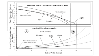
| Figure 1: Wage Curves and The Price of Corn for the Fluke Case |
This post extends a previous post. I am basically introducing structural dynamics into an example, by Bidard and Klimovsky of fake switch points.
At a rate of profits of zero in the example, the price of corn is zero for Alpha, one of the two techniques that is cost-minimizing there and for somewhat higher rates of profits. At a time before the fluke case, only the Gamma technique is cost-minimizing at a rate of profits of zero. The price of corn, as calculated with the Alpha technique, is negative at a rate of profits of zero. Alpha prices become non-negative only for positive rates of profits. This possibility cannot arise in examples with only single production and the choice of technique analyzed by the construction of the wage frontier.
2.0 A Fluke CaseTechnology and techniques are specified as in the previous post. I consider variations in labor coefficients with time. Two commodities can be produced jointly with each of three production process. In each process, workers produce outputs of the two commodities from smaller inputs of each commodities. Requirements of use are such that at least two processes must be operated. So each technique combines two processes.
A system of price equations is associated with each technique. The system, including an equation specifying the numeraire, can be taken to define the wage and the prices of both commodities, given an exogenous specification of the rates of profits. Table 1, at the head of this post, illustrates the solution prices at a given point of time. Linen is taken as the numeraire. The top half of the figure shows the wage, for each technique, as a function of the rate of profits. The bottom half of diagram shows the corresponding price of corn. Notice that, for the Alpha technique, the price of corn is zero when the rate of profits is zero.
A technique is only feasible, for the analysis of the choice of technique, when both the wage and prices are non-negative. In Figure 1, the rate of profits is partitioned into two roman-numbered regions. In Region II, both the Alpha and Gamma techniques are feasible. In Region III, only the Alpha technique is feasible.
At a switch point:
- The wage curves for at least two techniques intersect at the switch point.
- No extra profits can be made at the going rate of profits in any process.
- No excess costs arise for any process that can be operated at the switch point.
No switch points exist in the example at the time illustrated in Figure 1. For the structure of the example, all three wage curves intersect at a (non-fake) switch point. Furthermore, the price of corn is the same for all three techniques at the switching rate of profits.
Not enough information has been given so far to determine which techniques are cost-minimizing at each feasible rate of profits in Figure 1. I like to plot extra profits for each process and each price system. I do not show such plots in the post. Nevertheless, Table 1 summarizes which techniques are cost minimizing.
| Regions | Cost-Minimizing Technique | Processes |
| I | Gamma | b, c |
| II | Alpha and Gamma | a, b, c |
| III | Alpha | a, c |
Consider time before the fluke case illustrated in Figure 1. Labor coefficients are larger. Figure 2, below, illustrates the wage and price curves for a specified time before the fluke case described above. Notice the appearance of Region I, where Gamma is uniquely cost-minimizing. The fluke case is a knife-edge case where Region disappears. The wage axis becomes the boundary between Regions I and II. Of these two regions, only Region II exists for a positive rate of profits.

|
| Figure 2: A Fluke Fake Switch Point? |
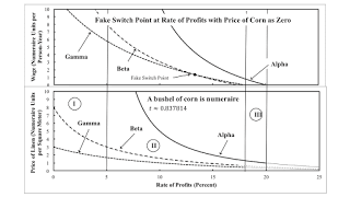
Does Figure 2 illustrate another fluke case? At the fake switch point at a rate of profits of five percent, the price of corn is zero. But consider Figure 3 below. The only difference in the example between Figures 2 and 3 is the specification of the numeraire. With corn as numeraire, the fake switch points disappear, and a new fake switch point appears at a rate of profits of 13 1/3 percent. The wage and the price of linen approach an asymptote for the rate of profits at which the price of corn is zero when linen is the numeraire. Which techniques are cost-minimizing is unaffected by the choice of the numeraire.

|
| Figure 3: Not A Fluke With Corn As Numeraire |
Consider some time after the fluke case illustrated in Figure 1. With the chosen parameters, labor coefficients have decreased less in the first production process than in the other two. Figure 4 shows the next qualitative change in the example, in which a switch point appears over the wage axis. I have already analyzed this case for this example.

|
| Figure 4: A Switch Point On The Wage Axis |
Between the times illustrated by Figures 1 and 4, Regions II and III continue to characterize the range of feasible non-negative rates of profits. The price of corn is positive, for all three techniques, is positive for feasible rates of profits for each technique. Region I has vanished.
The switch point continues to exist after the time illustrated in Figure 4, but at a positive rate of profits. A new region appears. For a rate of profits of zero and small positive rates of profits, the Beta technique is uniquely cost-minimizing.
5.0 ConclusionThis post has presented a fluke case only possible under joint production. In this example, the choice of technique cannot be determined by constructing the wage frontier.
This post has also presented a sort-of fluke case associated with a fake switch point. In this case, the fake switch point appears on the frontier at a rate of profits at which the price of corn is zero. The set of cost-minimizing techniques and processes varies at the fake switch point. But its existence depends on the choice of the numeraire.
I have been working on a taxonomy of fluke switch points for understanding structural economic dynamics. This post illustrates that my approach can extend to joint production. New phenomena and fluke cases can arise, and one must, perhaps, pay closer attention to what is and is not dependent on the choice of the numeraire.
 Heterodox
