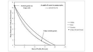
Figure 1: Wage Curves with Corn as Numeraire1.0 Introduction This post presents an example of a fluke switch point in which the choice of technique cannot be analyzed by the construction of the wage frontier. Under joint production, the technique that is cost-minimizing, for a given rate of profits, does not necessarily maximize the wage. Nevertheless, one can still see what I call a pattern over the wage axis in this case. The example is a generalization of the numerical example in Bidard & Klimovsky (2004). 2.0 Technology I postulate an economy in which two commodities, corn and linen, can be produced from inputs of corn, linen, and labor. Managers of firms know of three processes (Tables 1 and 2) to produce corn and linen. Each process produces net outputs of corn and linen as a
Topics:
Robert Vienneau considers the following as important: Example in Mathematical Economics, Joint Production
This could be interesting, too:
Robert Vienneau writes Austrian Capital Theory And Triple-Switching In The Corn-Tractor Model
Robert Vienneau writes Double Fluke Cases For Triple-Switching In The Corn-Tractor Model
Robert Vienneau writes The Emergence of Triple Switching and the Rarity of Reswitching Explained
Robert Vienneau writes Recap For A Triple -Switching Example
|
| Figure 1: Wage Curves with Corn as Numeraire |
This post presents an example of a fluke switch point in which the choice of technique cannot be analyzed by the construction of the wage frontier. Under joint production, the technique that is cost-minimizing, for a given rate of profits, does not necessarily maximize the wage. Nevertheless, one can still see what I call a pattern over the wage axis in this case. The example is a generalization of the numerical example in Bidard & Klimovsky (2004).
2.0 TechnologyI postulate an economy in which two commodities, corn and linen, can be produced from inputs of corn, linen, and labor. Managers of firms know of three processes (Tables 1 and 2) to produce corn and linen. Each process produces net outputs of corn and linen as a joint product. Inputs and outputs are specified in physical units (say, bushels and square meters) per unit level of operation of the given process. Inputs are acquired at the start of the year, and outputs are available for sale at the end of the year.
| Input | Process | ||
| (a) | (b) | (c) | |
| Labor | eσ0,1(1 - t) | eσ0,2(1 - t) | eσ0,3(1 - t) |
| Corn | 20 | 20 | 30 |
| Linen | 20 | 20 | 30 |
| Output | Process | ||
| (a) | (b) | (c) | |
| Corn | 21 | 23 | 36 |
| Linen | 27 | 25 | 34 |
I assume that requirements for use are such that two processes must be operated to satisfy those requirements. I need to investigate the implications of this assumption further. Apparently, for this example, it implies that the economy is not on a golden rule steady state growth path, with the rate of profits equal to the rate of growth. Anyway, with this assumption, three techniques - Alpha, Beta, and Gamma - can be operated. Table 3 specifies which processes are operated for each technique.
| Techniques | Processes |
| Alpha | a, b |
| Beta | a, c |
| Gamma | b, c |
The technology, as I have defined it, is parameterized. I consider the following specification for the rate of decrease in labor coefficients.
σ0,1 = 2
σ0,2 = σ0,3 = 5/2
Bidard & Klimovsky's example arises when t is unity. I consider the following value for time:
t ≈ 0.91973
Structural economic dynamics arises as time varies.
3.0 Price SystemPrices of production arise for each technique and each specification of the numeraire. For the Alpha technique, prices of production are characterized by the system of the following three equations:
(20 p1 + 20 p2)(1 + r) + [ eσ0,1(1 - t) ] w = 21 p1 + 27 p2
(20 p1 + 20 p2)(1 + r) + [ eσ0,2(1 - t) ] w = 23 p1 + 25 p2
p1d1 + p2d2 = 1
where:
- r is the rate of profits.
- w is the wage.
- p1 is the price of corn.
- p2 is the price of linen.
- d1 is the quantity of corn in the consumption basket serving as numeraire.
- d2 is the quantity of linen in the consumption basket serving as numeraire.
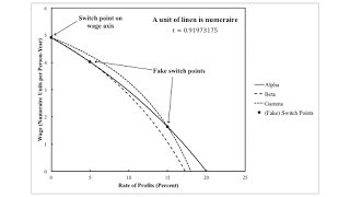
Given one of the distributive variables, this system of equations can be solved. Figure 1, at the top of this post, graphs the wage curves for the three techniques, when d1 = 1 and d2 = 0. Figure 2 graphs the wage curves when linen is the numeraire.
|
| Figure 2: Wage Curves with Linen as Numeraire |
Notice that which technique lies on the outer envelope, as the rate of profit, varies with the choice of numeraire. In Figure 1, the Alpha technique maximizes the wage, for all feasible positive rates of profits. In Figure 2, the Gamma technique, then the Alpha technique, maximizes the wage, with an increasing rate of profits. This dependence of qualitative characteristics of the wage frontier cannot arise when all capital goods are circulating capital.
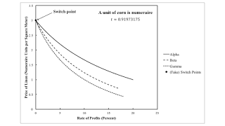
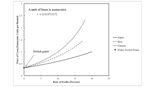
In the example, the two processes for a technique and the remaining process must all obtain the same rate of profits at a (genuine, non-fake) switch point. In the example, all three wage curves must intersect at a switch point. Another aspect of a switch point is that the prices of each good must be invariant across the price systems for the techniques entering the switch point. When corn is the numeraire, the price of linen must be the same for all three techniques at the switch point. This property is illustrated in Figure 3. The corresponding property for the price of corn, when linen is the numeraire, is illustrated in Figure 4. No sign of the fake switch points appears in Figures 3 and 4.
|
| Figure 3: Price of Linen with Corn as Numeraire |
|
| Figure 4: Price of Corn with Linen as Numeraire |
Wage curves can be misleading when analyzing the choice of technique under models of joint production. How then should the choice of technique be found?
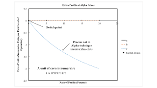
First, suppose the Alpha technique has been adopted. One can cost up the outputs and inputs of each process, for the solution to the price system for the Alpha technique. Figure 5 shows results. No extra profits, sometimes called pure economic profits, are made in operating the processes comprising the Alpha technique. For positive rates of profits, operating process c will not obtain the going rate of profits. Clearly, the Alpha technique is cost-minimizing for the graphed range of the rate of profits.
|
| Figure 5: Extra Profits with Alpha Prices |
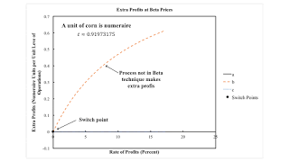
Second, suppose the Beta technique is chosen. Figure 6 graphs extra profits, for each process, as a function of the rate of profits, given Beta prices. For a positive rate of profits, the second process earns extra profits and will be adopted by managers of firms. Notice that one cannot tell from the diagram which process will be dropped. This issue does not arise without joint production. In the case of single production, only one process in the given technique produces the same commodity as that produced by the new process.
|
| Figure 6: Extra Profits with Beta Prices |
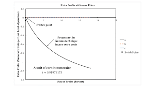
Finally, suppose the Gamma technique is chosen. Figure 7 graphs extra profits for this case. And the Gamma process is cost-minimizing for the full range of the rate of profits shown in the figure.
|
| Figure 7: Extra Profits with Gamma Prices |
The above has shown that, in this example, both the Alpha and Gamma techniques are cost-minimizing at feasible positive rates of profits. The Beta technique is cost-minimizing only at the switch point at a rate of profits of zero percent. The choice of technique is independent of the numeraire. Presumably, the choice between the Alpha and Gamma techniques is made based on requirements for use. At any rate, the chosen technique need not maximize the wage, given the rate rate of profits and the specification of the numeraire.
5.0 ConclusionThis example has illustrated that a specific fluke switch point, which I originally defined for cases with only circulating capital, can also arise in joint production. I except to find a need for new kinds of fluke switch points as I further examine joint production. I am hoping to be able to draw pattern diagrams in which qualitative properties are independent of the choice of the numeraire.
References- Bidard, Christian and Edith Klimovsky (2004). Switches and fake switches in methods of production. Cambridge Journal of Economics. 28 (1): 89-97.
 Heterodox
