Figure 1: APP Around Switch Points1.0 Introduction I take it that the Austrian theory of the business cycle builds on Austrian capital theory. The following two claims are central to Austrian capital theory: Given technology, profit maximizing firms adopt a more capital-intensive, more roundabout technique at a lower interest rate. The adoption of a more roundabout technique increases output per worker. Originally, Eugen von Böhm-Bawerk proposed a physical measure of the average period of production, but economists of the Austrian school have been distancing themselves from this position for well over half a century. I have argued that the first claim fails, even in a framework without any scalar measure of capital-intensity or the average period of production. Recently, Nicholas
Topics:
Robert Vienneau considers the following as important: Austrian School Of Economics, Example in Mathematical Economics, Sraffa Effects
This could be interesting, too:
Robert Vienneau writes Austrian Capital Theory And Triple-Switching In The Corn-Tractor Model
Robert Vienneau writes Double Fluke Cases For Triple-Switching In The Corn-Tractor Model
Robert Vienneau writes The Emergence of Triple Switching and the Rarity of Reswitching Explained
Robert Vienneau writes Recap For A Triple -Switching Example
|
| Figure 1: APP Around Switch Points |
I take it that the Austrian theory of the business cycle builds on Austrian capital theory. The following two claims are central to Austrian capital theory:
- Given technology, profit maximizing firms adopt a more capital-intensive, more roundabout technique at a lower interest rate.
- The adoption of a more roundabout technique increases output per worker.
Originally, Eugen von Böhm-Bawerk proposed a physical measure of the average period of production, but economists of the Austrian school have been distancing themselves from this position for well over half a century. I have argued that the first claim fails, even in a framework without any scalar measure of capital-intensity or the average period of production.
Recently, Nicholas Cachanosky and Peter Lewin, in a series of articles, have championed J. R. Hicks' measure of the Average Period of Production (APP), as a justification of the first claim. They note that the APP, as defined here, is a function of the interest rate. Hence, it cannot fully support Böhm-Bawerk's theory. Saverio Fratini has argued this justification does not work, since the second claim above fails, when this APP is used as a measure of capital-intensity. Lewin and Cachanosky, in reply, argue that Fratini does not properly calculate the APP, since it should be forward looking and apply in disequilibria.
This post re-iterates Fratini's argument, with his example. I more closely follow Cachanosky and Lewin's approach, though.
2.0 TechnologyFratini considers a technology consisting of two techniques of production, Alpha and Beta (Table 1). Each technique requires three years of unassisted labor inputs, per bushel wheat produced at the end of the third year. Labor is advanced and paid at the end of the year. Labor is taken as numeraire. That is, the wage is assumed to be $1 per person-year. The price of a bushel wheat, p, is taken to be $12 dollars per bushel. As I hope becomes apparent, these assumptions generally characterize a disequilibrium.
| Year | Years Until Harvest | Technique | |
| Alpha | Beta | ||
| 1 | 3 | a3 = 1 Person-Yr. | b3 = 8 Person-Yrs. |
| 2 | 2 | a2 = 7 Person-Yrs. | b2 = 2 Person-Yrs. |
| 3 | 1 | a2 = 2 Person-Yrs. | b1 = 2 Person-Yrs. |
The output per worker, in a stationary state, is determined by the chosen technique. Suppose the Alpha technique is adopted. In any given year, 10 person-years are employed per bushel wheat produced. Two person-years are being expended to produce each bushel of wheat harvested at the end of the year, seven person-years are being employed to produce each bushel of wheat available at the end of the next year, and one person-year is employed per bushel wheat harvested even a year later. That is, output per worker, under the alpha technique, yα, is (1/10) bushels per person-year. Similarly, output per worker for the beta technique, yβ, is (1/12) bushels per person-year.
3.0 Net Present Value and the Choice of TechniqueSuppose a wheat-producing firm faces a given annual interest rate, r. For convenience, define:
R = 1 + r
The discount factor, f, is defined to be:
f = 1/R = 1/(1 + r)
Consider a decision to choose a technique to adopt for next three years in producing wheat. Powers of the discount factor are used to evaluate the costs and revenues for each technique at the start of the given year. For example, the NPV of the alpha technique is:
NPV(α, f) = -a3f - a2f2 + (p - a1) f3
I have assumed that firms expect the given interest rate to remain unchanged for the decision period - a common convention. Revenues are positive, and costs (or outgoes) are negative.
Figure 2 graphs the difference between the NPV for the two techniques. A positive difference indicates that the alpha technique maximizes the NPV, while a negative difference arises when the beta technique is preferred. Which technique is chosen by cost-minimizing firm for each interest rate is shown. At switch points, firms are indifferent between the two techniques.

|
| Figure 2: Difference in NPVs |
Under the assumptions, NPV is always positive. (If the beta technique were adopted at an interest rate of zero, its NPV would be zero then.) If markets were competitive, the price of wheat would vary until the NPV was zero, given the interest rate. Fratini does indeed assume equilibrium and analyzes the choice of technique with backwards-looking calculations of costs, as Lewin and Cachanosky claim. But this makes no difference to his argument, so far.
4.0 The Average Period of ProductionOne might be interested in how NPV varies with the discount factor. The elasticity of the NPV, with respect to the discount factor, is a dimension-less number for assessing such sensitivity. Somewhat arbitrarily, I discount elasticity one period:
APP(α, f) = f [1/NPV(α, f)] [d NPV(α, f)/df]
Elasticity is the variation of NPV with variation of the discount factor, as a proportion of NPV.
APP(α, f) = [-a3f/NPV(α, f)] x 1+ [- a2f2/NPV(α, f)] x 2+ [(p - a1) f3/NPV(α, f)] x 3
The APP for a technique, at a given discount factor, is the weighted average of the time indices, looking forward, for a given income stream. The weights are the proportion of the income stream received in each period. All income is discounted to the start of the first year.
So the elasticity of the NPV of an income stream, with respect to the discount factor can also be expressed as the average period of production.
Notice that the APP is not defined in equilibrium. The denominators in the above terms are zero, and the APP could be said to be infinite. If only costs are used in the above calculations (thus, no longer of a NPV), the APP is well-defined, at least in the flow-input, point output case. Fratini (2019) does this.
One could also express the APP as a function of the interest rate:
APP(α, r) = [-a3R2/NPV(α, r)] x 1+ [- a2R/NPV(α, r)] x 2+ [(p - a1)/NPV(α, r)] x 3
where:
NPV(α, r) = -a3R2 - a2R + (p - a1)
I skip over some some algebraic manipulations above.
The above is not the definition of the APP in Fratini (2019), for example, in Equation 7. Where I have time indices of 1, 2, and 3, Fratini has indices of 3, 2, 1. I guess one can say that his definition of the APP is backwards-looking.
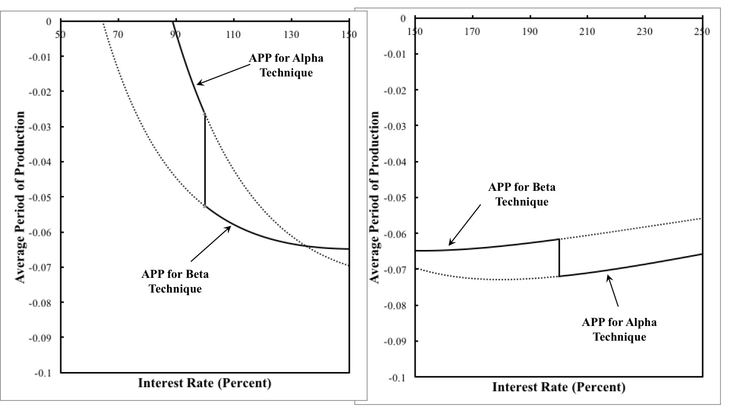
Fratini's argument still goes forward with Cachanosky and Lewin's (or Hicks') definition. One could present a mathematical proof that the APP is always increased around a switch point with a fall in the interest rate. But here I'll just graph it for the example. See Figure 1, at the top of this post. Around each switch point a lower interest rate is indeed associated with the adoption of a technique with a larger APP. But consider the switch point at an interest rate of 200 percent. The beta technique, adopted at a notionally lower interest rate, has a lower value of output per head.
4.0 ConclusionThe example illustrates that, around a switch point, a lower interest rate is associated with the adoption of a more roundabout technique, where roundaboutness is measured by Hicks' Average Period of Production. Incidentally, the example demonstrates that in a region where one technique is cost-minimizing the APP may decrease with the interest rate. But the adoption of a more roundabout technique can be associated with a decrease in output per worker. So much for Austrian capital theory and the Austrian theory of the business cycle.
References- Nicholas Cachanosky and Peter Lewin. 2014. Roundaboutness is not a mysterious Concept: A financial application to capital-Theory. Review of Political Economy, 26(4): 648-665.
- Saverio M. Fratini. 2019. A note on re-switching, the average period of production and the Austrian business-cycle theory, Review of Austrian Economics.
- J. R. Hicks. 1946. Value and Capital: An inquiry into some fundamental principles of economic theory. Oxford University Press.
- Peter Lewin. 1999. Capital in Disequilibrium: The role of capital in a changing world. Routledge.
- Peter Lewin and Nicholas Cachanosky. 2019. Re-switching, the average period of production and the Austrian business-cycle theory: A comment on Fratini, Review of Austrian Economics.