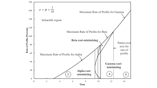
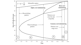
Figure 1: A Two-Dimensional Pattern Diagram, Enlarged1.0 Introduction This post further generalizes an example from Salvatore Baldone.. Like an example from Bertram Schefold, I find that Baldone's example is in a wedge near the edge of the appropriate region in one of my partitions of a parameter space. I have some very complicated spreadsheets that allow me to quickly visualize the effects of varying parameters. Baldone and Schefold were working long before Visicalc, Microsoft Excel, or LibreOffice. Finding these numeric examples must have been tedious. I think Baldone created this example to illustrate recurrence of truncation. Recurrence of truncation does not necessarily require the recurrence of techniques, but in this example recurrence of truncation occurs with recurrence of
Topics:
Robert Vienneau considers the following as important: Austrian School Of Economics, Example in Mathematical Economics, Joint Production, Sraffa Effects
This could be interesting, too:
Robert Vienneau writes Austrian Capital Theory And Triple-Switching In The Corn-Tractor Model
Robert Vienneau writes Double Fluke Cases For Triple-Switching In The Corn-Tractor Model
Robert Vienneau writes The Emergence of Triple Switching and the Rarity of Reswitching Explained
Robert Vienneau writes Recap For A Triple -Switching Example
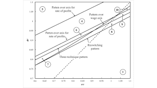
| Figure 1: A Two-Dimensional Pattern Diagram, Enlarged |
This post further generalizes an example from Salvatore Baldone.. Like an example from Bertram Schefold, I find that Baldone's example is in a wedge near the edge of the appropriate region in one of my partitions of a parameter space. I have some very complicated spreadsheets that allow me to quickly visualize the effects of varying parameters. Baldone and Schefold were working long before Visicalc, Microsoft Excel, or LibreOffice. Finding these numeric examples must have been tedious.
I think Baldone created this example to illustrate recurrence of truncation. Recurrence of truncation does not necessarily require the recurrence of techniques, but in this example recurrence of truncation occurs with recurrence of techniques. I found it interesting that I could also find here a non-monotonic variation of the economic life of a machine, without recurrence of techniques or capital-reversing.
2.0 TechnologyTables 1 and 2 specify the processes available in this economy. In the first process, labor works with corn to produce a new machine. In the remaining three processes, labor works with corn and a machine to produce corn. A machine one year older than the machine used as an input is jointly produced with corn. Prices of production are defined for coefficients of production at a given moment in time. Technical progress leads to coefficients of production for inputs declining over time. The notation allows for technical progress to be at different rates in the machine and corn sectors.
| Input | Process | |||
| (I) | (II) | (III) | (IV) | |
| Labor | (2/5) e1 - σ t | (1/5) e1 - φ t | (3/5) e1 - φ t | (2/5) e1 - φ t |
| Corn | (1/10) e1 - σ t | (2/5) e1 - φ t | 0.578 e1 - φ t | (3/5) e1 - φ t |
| New Machine | 0 | 1 | 0 | 0 |
| 1-Yr. Old Machine | 0 | 0 | 1 | 0 |
| 2-Yr. Old Machine | 0 | 0 | 0 | 1 |
| Output | Process | |||
| (I) | (II) | (III) | (IV) | |
| Corn | 0 | 1 | 1 | 1 |
| New Machine | 1 | 0 | 0 | 0 |
| 1-Yr. Old Machine | 0 | 1 | 0 | 0 |
| 2-Yr. Old Machine | 0 | 0 | 1 | 0 |
Three techniques of production exist here at each moment in time. I assume old machines can be discarded without cost. In the Alpha technique, machines are used for only one year. Old machines are used for two years in the Beta technique. In the Gamma technique, they are used for the full three years.
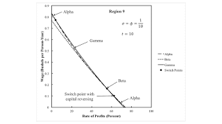
3.0 Prices of Production in Baldone ExampleI start by reproducing Baldone's example. I assume labor is advanced, and workers are paid a wage at the end of the year. Corn is taken as the numeraire. For each technique, one can solve for the wage and prices of machines as a function of the rate of profits. Figure 2 plots the wage curves for each technique. The cost-minimizing technique, at a given rate of profits, maximizes the wage. That is, the wage is on the outer envelope. It is not very visually obvious which technique is cost-minimizing, so I have labeled the cost-minimizing techniques. And one sees the Alpha is technique is cost minimizing at a low rate of profits. Around the switch point between the Alpha and Beta techniques, a higher wage is associated with the adoption of a more labor-intensive techniques.
| Figure 2: The Wage Frontier with the Recurrence of Techniques |
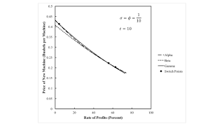
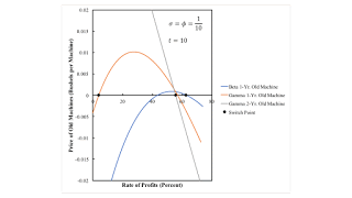
An aspect of the choice of technique can be seen by looking at prices. Figure 3 shows the price of new machines. For all techniques, the price of a new machine is positive for any feasible distribution. At a switch point, the price of a new machine is the same for both techniques that are cost-minimizing. Figure 4 shows how the price of old machines varies with the rate of profits. If a technique is cost-minimizing, the prices of old machines produced by that technique are non-negative at that rate of profits. At a switch point, the price of at least one produced old machine is zero. Baldone's article goes into much detail about prices of machines and truncation.
| Figure 3: The Price of a New Machine |
The price of an old machine is zero for a technique in which that machine is not produced. Figure 4 shows the prices of only those old machines that are produced in the corresponding technique. In an analysis of the choice of technique with fixed capital, if the price of an old machine is negative at a given rate of profits, the cost minimizing technique must have the economic life of machine must be truncated. Consider, for example, rates of profits less than approximately 4 percent or greater than approximately 63 percent. The price of a one-year old machine under the Beta technique is negative. The prices of one-year old and two-year old machines under the Gamma technique are both negative. Thus, neither can be cost-minimizing. The Alpha technique must be cost-minimizing in these ranges of the rates of profits.
| Figure 4: The Price of Old Machines in the Baldone Example |
I now take a first step in generalizing Baldone's capitalism. The rate of decrease of coefficients of production happens to be ten percent in both the machine and corn sectors. Figure 5 shows how the wage frontier varies with time under these assumptions. The maximum rate of profits and the rate of profits at switch points are plotted against time.
| Figure 5: Variation in the Wage Frontier with Time |
Here, the economy is not viable at the initial time. There must be some sort of low-productivity, backstop technology that was previously used. Figure 5 partitions time into six regions, and Figure 6 enlarges transient regions. Baldone's example is in Region 9.
| Figure 6: An Enlargement of the Variation in the Wage Frontier |
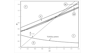
I now let the rates of decrease in coefficients of production differ between the machine and corn sector. Figure 7 graphs the resulting two-dimensional space and how it is partitioned by fluke switch points, which I call patterns. I only label one partition in Figure 7. For the partition between Region 0 and Region 1, the maximum rate of profits for the Alpha technique is zero, and the maximum rate of profits is negative for the Beta and Gamma techniques.
| Figure 7: A Two-Dimensional Pattern Diagram |
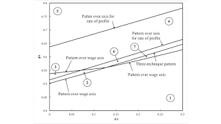
I look at two enlargements of parts ot the space in Figure 7 to get a somewhat more visually obvious understanding of what is going on here. Figure 8 is a blow-up of the middle left of Figure 7, and Figure 1 is a blow-up towards the middle right of Figure 7. I suppose I should say something more about this graph, but I will content myself with Table 3 and one observation. Consider the intersection of the boundaries between Regions 1 and 2, between 2 and 6, between 6 and 7, and between 7 and 1. This point is an intersection of three patterns over the wage axis with a three-technique pattern. I want to claim this intersection is generic, in some sense. I suppose precisely specifying in what sense would be publishable but maybe is beyond me.
| Figure 8: An Enlargement of the Parameter Space |
| Region | Technique | Summary |
| 0 | None | Not viable. |
| 1 | Alpha | No switch points. |
| 2 | Beta, Alpha | The switch point exhibits negative real Wicksell effects. A smaller rate of profits is associated with a longer economic life of a machine. |
| 3 | Beta | No switch points. |
| 4 | Gamma, Beta | The switch point exhibits negative real Wicksell effects. A smaller rate of profits is associated with a longer economic life of a machine. |
| 5 | Gamma | No switch points. |
| 6 | Gamma, Beta, Alpha | Switch points exhibit negative real Wicksell effects. A smaller rate of profits is associated with a longer economic life of a machine. |
| 7 | Gamma, Alpha | The switch point exhibits negative real Wicksell effects. A smaller rate of profits is associated with a longer economic life of a machine. |
| 8 | Alpha, Gamma, Alpha | The switch point at the higher rate of profits exhibits positive real Wicksell effects. Reswitching of techniques and recurrence of truncation. |
| 9 | Alpha, Gamma, Beta, Alpha | The switch point between Beta and Alpha exhibits positive real Wicksell effects. Recurrence of techniques and of truncation. |
| 10 | Alpha, Gamma, Beta | Switch points exhibit negative real Wicksell effects. A smaller rate of profits is associated with a non-monotonic variation in the economic life of machine. |
| 11 | Alpha, Gamma | The switch point exhibits negative real Wicksell effects. A smaller rate of profits is associated with a shorter economic life of a machine. |
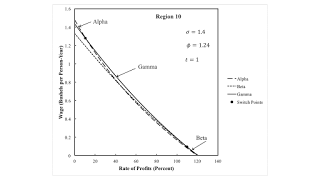
I might as well illustrate the wage frontier (Figure 9) in Region 10. From low to high wages (that is, high to low rates of profits) the cost-minimizing technique ranges from Beta through Gamma to Alpha. In a stationary state, the machine is run for two years at maximum rate of profits. At a middling rate of profits, its economic life is increased to three years. At an even lower rate, its economic life jumps down to one year. Around both switch points, corn produced per person-year is higher at the lower rate of profits. In some sense, the technique adopted at the lower rate of profits is more capital-intensive, despite the non-monotonic variation in the economic life of the machine. The switch point between Beta and Gamma is consistent with Austrian claims, but the switch point between Gamma and Alpha is a logical disproof of their capital theory.
| Figure 9: The Wage Frontier in Region 10 |
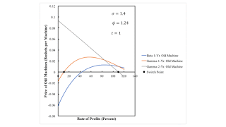
For completeness, Figure 10 plots the prices of produced old machines by technique. For a rate of profits below approximately 10.7 percent, the price of a one-year old machine is negative for both the Beta and Gamma techniques. Thus, neither is cost-minimizing in this range; the Alpha technique is. Between approximately 10.7 and 110 percent, the prices of both one-year old and two-year old machines is positive under the Gamma technique. It is not cost-minimizing to truncate the machine to one or two years in this range. For even larger feasible rates of profits, the price of a two-year old machine is negative under the Gamma technique, and the price of a one-year old machine is positive under the Beta technique. In this range, it is cost-minimizing to operate the machine for two years.
| Figure 10: Prices of Old Machines in Region 10 |
My methodology for generalizing Baldone's example leads to some complicated graphs. I find a couple of new phenomena that I have not seen in other examples of fixed capital. I think of Region 0, in which no specificed technique is viable. More interesting to me is Region 10, in which the economic life of a machine varies non-monotonically with the rate of profits, without either recurrence of techniques or cost-minimizing.
Reference- Salvatore Baldone. 1974. Il capitale fisso nello schema teorico di Piero Sraffa. Studi Economici XXIV(1): 45-106. Translated in Pasinetti (1980).
 Heterodox

