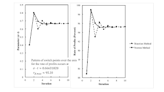
Figure 1: Convergence to a Pattern of Switch Points over the Axis for the Rate of Profits1.0 Introduction This post illustrates how to find fluke switch points. As usual, I proceed by example, in this case, as taken from my paper in Structural Change and Economic Dynamics. 2.0 Technoplogy In this example of a capitalist economy, two commodities, iron and corn, are produced. One process is known for producing iron. In the iron industry, workers use inputs of iron and corn to produce an output of iron. The output of the iron industry is one ton with the inputs shown in Table 1. Two processes are known for producing corn. Each corn-producing process shown in Table 1 produces an output of one bushel corn from inputs of labor power, iron, and corn. Assume constant returns to scale. Table
Topics:
Robert Vienneau considers the following as important: Example in Mathematical Economics, Protocols
This could be interesting, too:
Robert Vienneau writes Austrian Capital Theory And Triple-Switching In The Corn-Tractor Model
Robert Vienneau writes Double Fluke Cases For Triple-Switching In The Corn-Tractor Model
Robert Vienneau writes The Emergence of Triple Switching and the Rarity of Reswitching Explained
Robert Vienneau writes Recap For A Triple -Switching Example
| Figure 1: Convergence to a Pattern of Switch Points over the Axis for the Rate of Profits |
This post illustrates how to find fluke switch points. As usual, I proceed by example, in this case, as taken from my paper in Structural Change and Economic Dynamics.
2.0 TechnoplogyIn this example of a capitalist economy, two commodities, iron and corn, are produced. One process is known for producing iron. In the iron industry, workers use inputs of iron and corn to produce an output of iron. The output of the iron industry is one ton with the inputs shown in Table 1. Two processes are known for producing corn. Each corn-producing process shown in Table 1 produces an output of one bushel corn from inputs of labor power, iron, and corn. Assume constant returns to scale.
| Input | Industry | ||
| Iron | Corn | ||
| I | II Alpha | II Beta | |
| Labor | a0,1 = 1 | a0,2α = (5191/5770) e1/10 - σt | a0,2β = 305/494 |
| Iron | a1,1 = 9/20 | a1,2α = (1/40) e1/10 - σt | a1,2β = 3/1976 |
| Corn | a2,1 = 2 | a2,2α = (1/10) e1/10 - σt | a2,2β = 229/494 |
I take corn as the numeraire. Wages are paid out of the surplus at the end of the harvest. I take the rate of profits as given. In this post, I do not explain how to find the price of iron and the wage for, say, the Alpha technique, given the technology at a given value of (σ t).
At a switch point, no excess profits or costs arise in evaluating the Beta process in the corn industry at Alpha prices. That is, switch points are the roots of the following equation.
1 - {[p1α(σt) a1,2β + a2,2β](1 + r) + wα(σt) a0,2β} = 0
The above is a quadratic equation for this example. Let fk(σ t) denote the kth root of the above equation.
rk = fk(σ t)
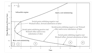
These are the switch points for a specific value of the parameters σ t. I fix σ at 1/10. Figure 2 graphs the switch points, as well as the maxmimum wage, against time. You can see technical progress brings about reswitching and takes it away.
| Figure 2: Fluke Switch Points Partition Time |
Various fluke cases arise in the example. They can be found by numerical methods. Table 2 defines, for four types of fluke cases, a new function whose root is the parameter values that correspond to the type of fluke case. For illustration, consider the fluke switch point that arises on the axis for the rate of profits with σ t ≈ 0.6663189. That is, g(σ t) is the difference between the maximum rate of profits for the Beta technique and the rate of profits for a selected switch point for the Alpha and Beta techniques.
| Function | Fluke Case |
| gk(σ t) = fk(σ t) + 1 | Pattern of switch points for the reverse substitution of labor. |
| gk(σ t) = fk(σ t) | Pattern of Switch points over the wage axis. |
| gk(σ t) = rmax, β - fk(σ t) | Pattern of switch points over the axis for the rate of profits. |
| gk(σ t) is the discriminant of the quadratic equation above | Reswitching pattern of switch points. |
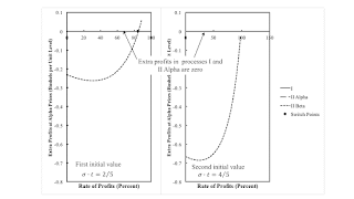
One needs two initial parameter values to start either algorithm specified here. Figure 3 graphs extra profits in operating the corn process in the Beta technique, as evaluated at Alpha prices. Extra profits are shown for two different parameter values. On the left panel, a switch point exists for a rate of profits smaller than the maximum rate of profits. The parameter values are evidently too small for a pattern of switch points over the axis for the rate of profits. On the right panel, the parameter values are too large. These are acceptable initial values.
| Figure 3: Initial Values for a Pattern Over the Axis for the Rate of Profits |
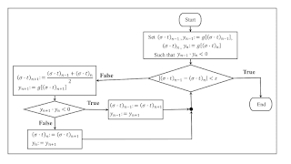
One can find the desired parameter value by either a bisection method or Newton’s method. Figure 4 provides a flowchart for the bisection method. The parameter values are updated to the midpoint of the current iterations. One of the current iterations is updated while keeping invariant the condition that the current iterations bound the zero of the function whose zero is sought. When the distance between the current iterations is small enough, either iteration is considered an acceptable approximation of the parameter values at which the fluke case arises.
| Figure 4: Bisection Method |
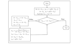
Figure 5 specifies Newton's method. An iteration for Newton’s method is based on approximating the function whose zero is sought by a straight line going through the two points determined by the previous two iterations. You can see that the slope and intercept for this line are found in the block in the lower left of the figure. And that the next iteration of the parameter values are found by an update calculated with this slope and intercept.
| Figure 5: Newton Method |
Newton's method is not guaranteed to converge, albeit I have had no issues in this context of finding fluke cases in the analysis of the choice of technique. When it does converge, its convergence is much faster than the bisection method (Figure 1).
 Heterodox

