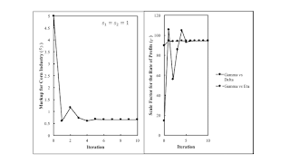
Figure 1: Convergence of Newton Method This post steps through an algorithm for finding a fluke switch point. I used a different example when I tried to explain this before. Today, I use an example building on my draft ROPE Article. Consider Figure 3 in this post, repeated below as Figure 2. Let s1 = s2 = 1. I want to find s3, the markup in the corn industry, such that the wage curves for Gamma, Delta, Eta, and Theta intersect at a single switch point. One wants to find a function one of whose zeros is the desired markup. Figure 2: Variation of Switch Points with the Markup in the Corn Industry This economy produces a single consumption good, called corn. Corn is also a capital good, that is, a produced commodity used in the production of other commodities. In fact, iron, steel, and
Topics:
Robert Vienneau considers the following as important: Example in Mathematical Economics, Full Cost Prices, Protocols
This could be interesting, too:
Robert Vienneau writes Austrian Capital Theory And Triple-Switching In The Corn-Tractor Model
Robert Vienneau writes Double Fluke Cases For Triple-Switching In The Corn-Tractor Model
Robert Vienneau writes The Emergence of Triple Switching and the Rarity of Reswitching Explained
Robert Vienneau writes Recap For A Triple -Switching Example
| Figure 1: Convergence of Newton Method |
This post steps through an algorithm for finding a fluke switch point. I used a different example when I tried to explain this before. Today, I use an example building on my draft ROPE Article.
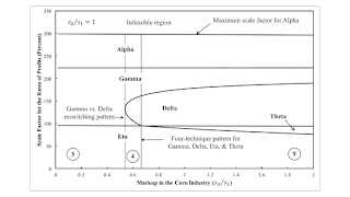
Consider Figure 3 in this post, repeated below as Figure 2. Let s1 = s2 = 1. I want to find s3, the markup in the corn industry, such that the wage curves for Gamma, Delta, Eta, and Theta intersect at a single switch point. One wants to find a function one of whose zeros is the desired markup.
| Figure 2: Variation of Switch Points with the Markup in the Corn Industry |
This economy produces a single consumption good, called corn. Corn is also a capital good, that is, a produced commodity used in the production of other commodities. In fact, iron, steel, and corn are capital goods in this example. So three industries exist. One produces iron, another produces steel, and the last produces corn. Two processes exist in each industry for producing the output of that industry. Each process exhibits Constant Returns to Scale (CRS) and is characterized by coefficients of production. Coefficients of production (Table 1) specify the physical quantities of inputs required to produce a unit output in the specified industry. All processes require a year to complete, and the inputs of iron, steel, and corn are all consumed over the year in providing their services so as to yield output at the end of the year.
| Input | Iron Industry | Steel Industry | Corn Industry | |||
| a | b | c | d | e | f | |
| Labor | 1/3 | 1/10 | 5/2 | 7/20 | 1 | 3/2 |
| Iron | 1/6 | 2/5 | 1/200 | 1/100 | 1 | 0 |
| Steel | 1/200 | 1/400 | 1/4 | 3/10 | 0 | 1/4 |
| Corn | 1/300 | 1/300 | 1/300 | 0 | 0 | 0 |
A technique consists of a process in each industry. Table 2 specifies the eight techniques that can be formed from the processes specified by the technology. If you work through this example, you will find that to produce a net output of one bushel corn, inputs of iron, steel, and corn all need to be produced to reproduce the capital goods used up in producing that bushel.
| Technique | Processes |
| Alpha | a, c, e |
| Beta | a, c, f |
| Gamma | a, d, e |
| Delta | a, d, f |
| Epsilon | b, c, e |
| Zeta | b, c, f |
| Eta | b, d, e |
| Theta | b, d, f |
Given the markups s1, s2, and s3, the wage and prices under Gamma are rational functions of the scale factor for the rate of profits:
wγ(r) = (f3r3 + f2r2 + f1r + f0)/(g2r2 + g1r + g0)
pγ,1(r) = (u2r2 + u1r + u0)/(g2r2 + g1r + g0)
pγ,2(r) = (v2r2 + v1r + v0)/(g2r2 + g1r + g0)
Since corn is the numeraire, its price is unity. The coefficients of the polynomials are functions of the coefficients of production for the first, second, and first processes in the iron, steel, and corn industries, respectively, and of the markups.
The Delta technique differs from Gamma in the process for producing corn. The extra profits obtained in operating the second corn-producing process at Gamma prices are:
h1(r)/(g2r2 + g1r + g0) = 1- [(af,1,3pγ,1(r) + af,2,3pγ,2(r) + af,3,3)(1 + s3r)+ af,0,3wγ(r)]
A switch point between Gamma and Delta is found as an appropriate zero of h1(r), which is a cubic polynomial. Denote r1(s3) as the zero sought for the fluke case.
The extra profits obtained in operating the second iron-producing process at Gamma prices are:
h2(r)/(g2r2 + g1r + g0) = pγ,1(r)- [(ab,1,1pγ,1(r) + ab,2,1pγ,2(r) + ab,3,1)(1 + s1r)+ ab,0,1wγ(r)]
An appropriate zero of h2(r) is a switch point between Gamma and Eta. Denote r2(s3) as the zero sought for the fluke case.
Consider the following function:
h(s3) = r2(s3) - r1(s3)
A zero of h(s3) is such that the wage curves for Gamma, Delta, Eta, and Theta intersect at a single switch point. At a switch point for Gamma, Delta, and Eta, neither extra profits nor extra costs will be obtained in operating either iron-producing and corn-producing processes. Since the same steel-producing process is operated in all four techniques, Theta is also cost-minimizing at this switch point.
One can find such a zero by applying Newton’s method to two initial guesses, as illustrated in Figure 1 at the top of the post. Some experimentation allows one to determine two initial guesses, s03 and s13, for the markup in the corn industry and for which roots of the cubics are wanted. The slope of a linear approximation to the function whose zero is sought is:
mi + 2 = [h(si3) - h(si + 13)]/(si3 - si + 13), i = 0, 1, 2, ...
The intercept with the ordinate is:
bi + 2 = h(si + 13 - mi + 2si + 13, i = 0, 1, 2, ...
The next iteration is:
si + 23 = - bi + 2/mi + 2, i = 0, 1, 2, ...
In my experience, Newton's method converges fairly rapidly in this application of finding fluke switch points.
 Heterodox


