In some recent posts, a job guarantee has been considered within the income-expenditure framework. One post in particular suggested a possible conceptualization of the dynamics of the model. It was shown that these dynamics are consistent with the model’s steady state requirements. Demonstrating this took a fair bit of algebra, which may have obscured for some readers the simplicity of the actual model. Much of the algebra was only needed for the specific purpose of verifying that the suggested dynamics are valid. At least for the version of the model presently under consideration, this task has now been accomplished. It is justifiable just to focus on the basic model which is really quite simple while still allowing for somewhat complicated behavior. Below, an example of this behavior
Topics:
peterc considers the following as important: Job & Income Guarantee
This could be interesting, too:
peterc writes Macro Dynamics with a Job Guarantee – Part 6: Price Stabilization
peterc writes Macro Dynamics with a Job Guarantee – Part 5: Price Level
peterc writes Macro Dynamics with a Job Guarantee – Part 4: Dynamic Stability
peterc writes Macro Dynamics with a Job Guarantee – Part 3: Adjustment Process
In some recent posts, a job guarantee has been considered within the income-expenditure framework. One post in particular suggested a possible conceptualization of the dynamics of the model. It was shown that these dynamics are consistent with the model’s steady state requirements. Demonstrating this took a fair bit of algebra, which may have obscured for some readers the simplicity of the actual model. Much of the algebra was only needed for the specific purpose of verifying that the suggested dynamics are valid. At least for the version of the model presently under consideration, this task has now been accomplished. It is justifiable just to focus on the basic model which is really quite simple while still allowing for somewhat complicated behavior. Below, an example of this behavior is provided. First, though, it seems worth putting things into context with a quick summary of the key variables and parameters.
Summary of the Model
Readers of the earlier post could be forgiven for thinking that the modified income-expenditure model introduces lots of new variables. Although it does involve some variables that are not explicitly included in the base model, there are actually very few new variables introduced. Those that are introduced are there because: (i) we are considering the composition of income in addition to its total level; and (ii) we are explicitly considering the level and composition of employment, whereas the level of employment is only implicit in the base model.
Basically, we have income variables, employment variables and demand variables. The income variables are total income Y, sector b income Yb and sector j income Yj. The corresponding employment variables are L, Lb and Lj. Partly compensating for the inclusion of sectoral income and employment variables, we have simplified the treatment of demand such that there are only autonomous demand A, induced household consumption net of endogenous imports CI and job guarantee spending Gj.
At this stage, only the income measures, sectoral employment levels, induced household consumption and job guarantee spending are endogenous variables. Autonomous demand and total employment are exogenous.
Anything else in the model is either a parameter (and so exogenously given) or a summary term involving the parameters. The parameters are the marginal propensity to leak α (equal to one minus the net marginal propensity to consume c), sector b productivity ρb, the job guarantee wage wj and the fraction of job guarantee spending going to wages ϕ (equal to one minus the fraction of job guarantee spending going to materials m). The summary terms are k, M, v and q. The first three of these relate to the dynamics about to be illustrated. The last summary term is job guarantee spending expressed as a fraction of the income gap.
Overview of the Dynamics
When income is fully adjusted to demand, the system is in a steady state. An exogenous change in demand disturbs the steady state. (The same is true of an exogenous change in total employment). On the basis of the suggested dynamics, the exogenous change in demand sets off an adjustment process that brings the system back to a steady state. This is true under all plausible values of the parameters.
The dynamics followed by the system are dictated by very simple recursive (difference) equations. In the initial time step, income and sector b income are assumed to respond by the amount of the exogenous change in demand. In the subsequent time step, consumption responds to the change in income in accordance with the net marginal propensity to consume and job guarantee spending adjusts by a fraction of the change in sector b income. These adjustments alter income and its composition in the same time step. This causes further adjustment in induced consumption and job guarantee spending at the next time step with immediate effects once again on income and its composition. The process continues until a steady state is restored.
This is certainly not the only way the dynamics could have been depicted. (I have experimented with a number of alternatives.) The choice was made mainly for a couple of reasons. First, the dynamics are analogous to the way the base model’s dynamics are typically interpreted, with endogenous spending adjusting to changing income with a lag. Second, even under present assumptions in which sector b productivity and the labor force participation rate are taken as given, there is likely to be a short lag in the response of job guarantee spending because of the existence of pay periods and payment schedules. For instance, if a worker switches from a job guarantee position to a role in the broader economy, the impact on income will precede the impact on job guarantee spending. The latter will be delayed because workers are usually paid at the end of a pay period rather than at the beginning. If we think of the time steps as fortnightly periods, then at time t = 0 there is an increase in autonomous demand with immediate impacts on income and its composition. Under present assumptions, this higher income can only be achieved through a transfer of some employment to sector b. At the end of the fortnight (time t = 1) these workers will be paid by sector b employers rather than receiving the job guarantee wage and at this point job guarantee spending will decrease.
Job Guarantee Spending
In a steady state, the level of job guarantee spending is
All terms on the right-hand side are exogenous variables or parameters (q is defined solely in terms of parameters).
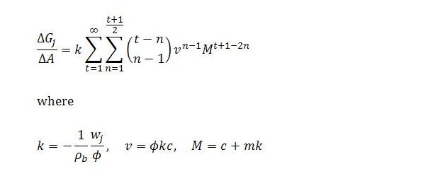
An exogenous change in demand will cause Gj to diverge from its steady state. Its adjustment is described by
This looks a lot scarier than it actually is. Suppose the net marginal propensity to consume is 1/2, sector b productivity is ρb = 2, the job guarantee wage is wj = 1/2 and the fraction of job guarantee spending going to wages is 2/3. This is all the information we need to work out the values of k, v and M and the change in job guarantee spending with respect to autonomous demand at each time step t and in total. The index n simply refers to the nth term in the equation for each time step.
In our example, k = 3/8, v = -1/8 and M = 3/8. In principle, the change in job guarantee spending can be calculated as
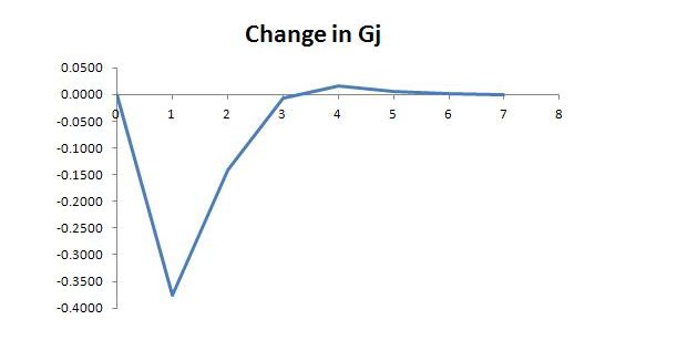
The changes for t = 1 to t = 10 (to four decimal places) are:
Although we are dealing with an infinite series, the total changes are pretty much spent at this point, being about 0.000014 away from the ultimate change, for which we possess a convenient formula:
This says that a one unit increase in autonomous demand ultimately causes job guarantee spending to decrease by half a unit.
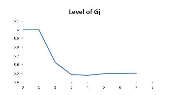
Graphically, the adjustment looks roughly as shown below (the software assumes a constant rate of change within each time step):
The graph showing the level of Gj over time is based on an initial level of autonomous demand of 88 and total employment of 100. The initial level of 6 compares with total income of 188. The final level of 5.5 compares with total income of 189.
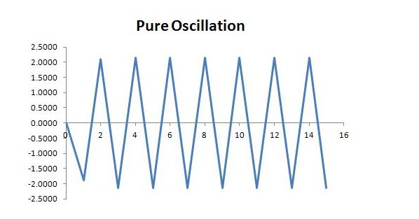
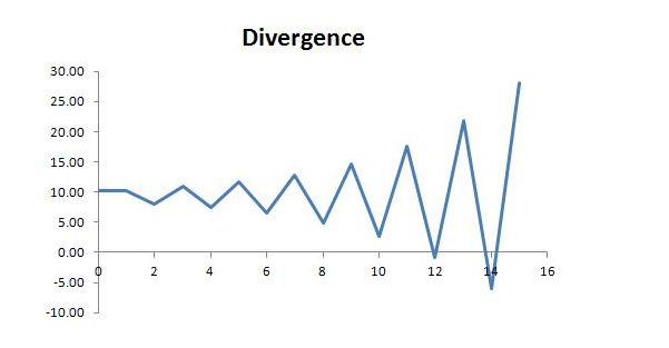
It was mentioned in the earlier post that convergence to a steady state is assured for plausible values of the parameters. It was also noted that, mathematically, divergence could occur if wages made up an unrealistically small fraction of job guarantee spending. For the fun of it, this is illustrated in the next two graphs. Holding all the other parameters at the same level, oscillation without a trend occurs if ϕ = 2/15 and divergence occurs for values of ϕ smaller than this (ϕ = 0.12 in the second graph).
Sector b Income
The behavior of the other endogenous variables can be considered in the same way. In what remains, we will mainly consider sector b income. In a steady state, the sector’s income satisfies
Once again, all terms on the right-hand side other than the summary term q are exogenous variables or parameters.
An exogenous change in demand will cause Yb to diverge from its steady state, with its adjustment process described by
Assuming the same parameter values as earlier we once again have k = 3/8, v = -1/8 and M = 3/8. In principle, the change in sector b income can be calculated as
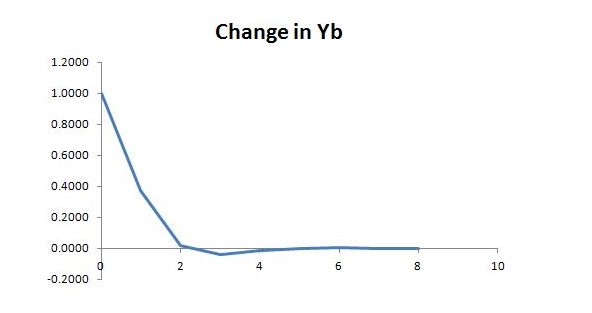
The changes for t = 0 to t = 9 are:
As before, the total changes are pretty much spent at this point. The ultimate change is given by the formula:
This says that a one unit increase in autonomous demand ultimately causes sector b income to rise by 4/3 units.
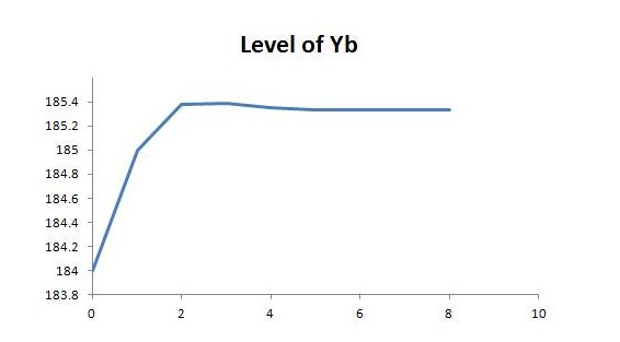
Graphically, the adjustment looks something like this:
As before, the graph showing the variable’s level is based on initial autonomous demand of 88 and total employment of 100. The initial level of 184 compares with total income of 188. The final level of 185 1/3 compares with total income of 189.
Other Variables
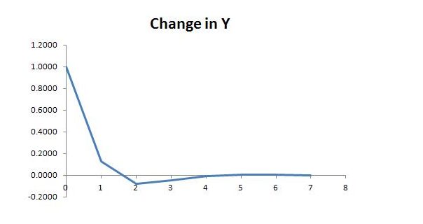
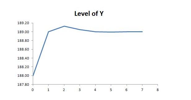
The behavior of total income and the other endogenous variables is in simple relation to the behavior of job guarantee spending and sector b income. In particular, the change in Y at time step t will be the change in sector b income plus ϕ times the change in job guarantee spending. Since job guarantee spending varies inversely to sector b income, the ultimate change in income is somewhat smaller than the corresponding impact on sector b income. The total change is
For the particular example we have considered, the behavior looks roughly like this:


