The model, in its present form, is short run in nature. It concerns an economy for which total employment, within-sector productivity and productive capacity are all taken as given. Variations in total output are achieved by workers transferring between two broad sectors that have differing productivity. In considering this economy, discussion has touched on aspects of a steady state and system behavior outside the steady state. It has been supposed, in the event of exogenous shocks, that the broader economy (sector b) drives the adjustment process through its reactions to excess demand or excess supply, with the job-guarantee program (sector j) absorbing or releasing workers as appropriate to maintain total employment at its given level. A tendency for the economy to move toward the
Topics:
peterc considers the following as important: Job & Income Guarantee
This could be interesting, too:
peterc writes Macro Dynamics with a Job Guarantee – Part 6: Price Stabilization
peterc writes Macro Dynamics with a Job Guarantee – Part 5: Price Level
peterc writes Macro Dynamics with a Job Guarantee – Part 3: Adjustment Process
peterc writes Macro Dynamics with a Job Guarantee – Part 2: Keynesian Cross Diagram
The model, in its present form, is short run in nature. It concerns an economy for which total employment, within-sector productivity and productive capacity are all taken as given. Variations in total output are achieved by workers transferring between two broad sectors that have differing productivity. In considering this economy, discussion has touched on aspects of a steady state and system behavior outside the steady state. It has been supposed, in the event of exogenous shocks, that the broader economy (sector b) drives the adjustment process through its reactions to excess demand or excess supply, with the job-guarantee program (sector j) absorbing or releasing workers as appropriate to maintain total employment at its given level. A tendency for the economy to move toward the steady state has been illustrated with reference to a Keynesian cross diagram (part 2) and a description of the growth behavior of actual output and demand whenever the system is outside the steady state (part 3). Attention now turns to the conditions under which this tendency to a steady state is operative, or, in other words, to the question of dynamic stability.
Dynamic stability, in the present context, requires that when the system is in a steady state, it has no inherent tendency to leave that state, and if an exogenous shock disturbs the system, the system’s tendency is to return to the steady state. It was noted in part 1 that a steady state can only occur if the share of job-guarantee spending in total income stabilizes at j = j*. This itself can only occur if the sectoral composition of employment stabilizes, with Lb = Lb* and Lj = Lj*. And, for the sectoral composition of employment to stabilize, sector b must have succeeded in eliminating any excess demand or excess supply so that there is no impetus for the sector’s output to change: Yb‘ = λ(Y – Yd) = 0. So long as there is no impetus for sector b output to change, there will likewise be no impetus for sector b employment to change (since within-sector productivity is taken as given), nor for sector j output or employment to change, nor for total output to change. The issue of dynamic stability therefore hinges on there being a tendency for actual output Y to adjust fully to total demand Yd and, once this has occurred, for the situation to persist in the absence of shocks.
Dynamic stability in a stationary economy
Establishing dynamic stability is straightforward in the simple version of the model currently under discussion. With autonomous demand, within-sector productivity and total employment all held constant, a situation in which total output is adjusted to total demand is not only a steady state but also a stationary one. In a stationary state, output and demand are both constant, as are the levels of all other variables.
It is necessary only to consider the behavior of total output over time. In part 3, this behavior was reduced to a simple differential equation which can be written in the form:

where Y’ is the time derivative of Y (dY/dt), Yd is total demand, Y is total output, λ is a parameter indicating the strength of sector b’s quantity response to excess demand, k is the absolute response of job-guarantee spending to a unit change in sector b output and q is the fraction of the output gap that is matched by job-guarantee spending. In the short run, λ, k and q are all taken to be constant. Substituting the demand function

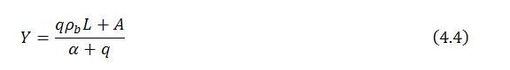
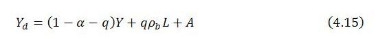
into (4.1) gives a linear first-order differential equation that relates the instantaneous change in total output to a single variable, the level of total output itself

with α representing the marginal propensity to leak, ρb productivity of the broader economy, L total employment and A autonomous demand.
In a steady state, Y’ = 0. This occurs when
which is the steady-state level of output Y*. This level of output depends only on given parameters and exogenous variables.
Local stability requires the derivative of Y’ with respect to Y to be negative when evaluated at the critical value Y = Y*. For a linear differential equation, this derivative is constant, meaning that the system is globally stable provided the derivative of Y’ with respect to Y is negative for all positive levels of output.

It clearly makes no difference where the derivative is evaluated because it takes the same value for all levels of output, depending only on given values of the parameters. Since these parameters all take positive values, the derivative is negative as required for global stability.
The situation is illustrated below:
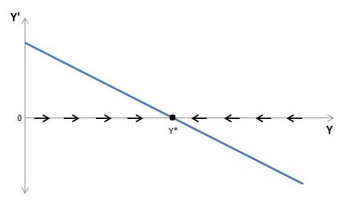
Whenever Y is below Y*, Y’ is positive so that Y rises toward Y*. Conversely, whenever Y is above Y*, Y’ is negative so that Y falls toward Y*.
In the present form of the model, then, the tendency is always for total output to move toward its steady-state level and, upon reaching the steady state, to remain there in the absence of further exogenous shocks.
A more general approach
It has been noted that the analysis of dynamic stability is often easier for systems that are stationary in the steady state. For systems that grow even when in the steady state, the evaluation of dynamic stability can get more involved. It is then no longer sufficient to consider the behavior of levels, because the levels of some key variables, such as total output, will not be constant in the steady state of a continually growing economy. The ‘steadiness’ of a state will instead need to be evaluated in relation to other measures, such as rates of growth or ratios between levels.
It may be instructive to introduce a more general approach to the analysis of dynamic stability now, while the model is relatively simple. This will illustrate how the issue of dynamic stability can be considered in terms of ratios and growth rates. The approach, which is not strictly necessary at the moment, leads to the same conclusion as reached in the previous section, but in a slightly different way.
A convenient option is to collapse demand and output into a single variable y. This variable has already been introduced in part 3 as an alternative measure of excess demand:

When viewed in terms of (4.6), a steady state requires that y = 1 and y’ = dy/dt = 0. Dynamic stability will pertain if whenever y deviates from 1, there is a tendency for it to return to 1 and stay there.
The first condition for a steady state, y = 1, is satisfied when actual output equals total demand. The second condition, y’ = 0, rules out instances where y = 1 only momentarily as actual output switches from being above total demand to below it, or vice versa.
Dynamic stability can be investigated by expressing y’ as a function of y and then considering the behavior of the function. In general terms, y’ depends upon y and the growth rates of total demand and total output (gd and g, respectively),

In the simplest version of the model, the growth rates of demand and output are
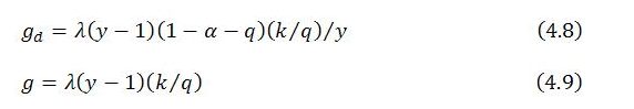
These growth equations are discussed in part 3. Substituting for gd and g in (4.7) enables y’ to be expressed as a function of just one variable, y:

This differential equation is non-linear. There are two critical values at which y’ = 0, specifically y = 1 and y = 1 – α – q. Local stability can be analyzed by considering a linear approximation to the non-linear behavior of the system at these two y-values. The behavior of the system at and near a critical value is inferred from the sign of the derivative of y’ with respect to y evaluated at that y-value. A negative sign indicates a point of local stability to which the system is attracted; a positive sign indicates a point of local instability from which the system is repelled:
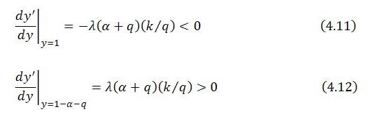
Local stability analysis therefore suggests that y = 1 is a point of stability and y = 1 – α – q is a point of instability. So long as y is “close” to 1, the system moves toward y = 1. If an exogenous shock placed y in the vicinity of 1 – α – q, the system would move away from that position. In short, y = 1 attracts the system, whereas y = 1 – α – q repels the system. These results are consistent with a tendency for the system to converge on the steady state provided y > 1 – α – q. However, if it were possible for an exogenous shock to plunge y below 1 – α – q, the system would be pushed away from both critical values toward zero, with the system imploding.
For non-linear behavior, it is often difficult to analyze dynamic stability other than through the linear approximation provided by local stability analysis. Under present assumptions, though, the model is sufficiently simple that stability can be assessed more directly by considering how, according to (4.10), the system behaves starting from any value of y. The two critical values,
![]()
suggest that there are three intervals of relevance when examining the system’s behavior:
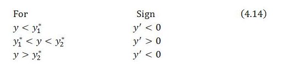
Consistent with what has been found through local stability analysis, the system is repelled by the first critical value (y = y1* = 1 – α – q) and attracted by the second critical value (y = y2* = 1). If the value of y could ever fall below 1 – α – q, y would tend toward zero, with economic activity collapsing. But so long as y is above 1 – α – q, y tends toward the second critical value y = 1 associated with the steady state. When y is above 1 – α – q but less than 1, y’ is positive and y rises toward 1. And when y is above 1, y’ is negative and y falls toward 1.
The system therefore tends toward the steady state provided y > 1 – α – q, as illustrated below:

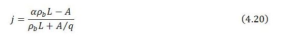
As might be guessed from the results already obtained in the previous section, under present assumptions the condition that y exceeds 1 – α – q is always satisfied. This can be seen by recalling that total demand takes the form
and noting that y itself can be expressed as

Since all the parameters and exogenous variables as well as total output are positive,

and the condition y > 1 – α – q always holds. This ensures that the system tends toward the steady state for all plausible values of the parameters.
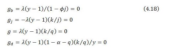
The behavior of other endogenous variables
It is not only y (or Y) that converges on a steady state. All the endogenous variables do the same through their participation in the system’s adjustment process. This can be verified by noting that when y = 1, which has already been shown to be a point of attraction for the system, all endogenous variables are in the steady state, and in fact stationary. In particular, when y = 1, all endogenous growth rates are zero:
Under the assumption of constant within-sector productivity, the zero growth rates of sectors b and j also imply constant sectoral employment levels and constant sectoral employment shares.
Lastly, consider the share of job-guarantee spending in income:

When total output is at its steady-state level Y = (qρbL + A)/(α + q),
which is constant at the steady-state value j = j*. Accordingly, j’ = 0, indicating that the share of job-guarantee spending in income is stable in the steady state.