The previous part of the series introduced a short-run relationship between prices and output, P(Y), that is in keeping with a Kaleckian or Keynesian understanding of demand-led economies. According to this view, within the economy’s capacity limits, output reflects demand while prices reflect cost. So long as supply conditions remain unaltered, variations in demand are met with variations in production at stable prices. But when spending goes beyond the economy’s current capacity to respond in quantity terms, price pressures emerge from the demand side. These considerations suggest a shape for P(Y) that is approximately horizontal over a ‘normal’ range of output centered on Yn but that is sharply increasing for output close to the maximum possible, Ymax. A policy implication is that
Topics:
peterc considers the following as important: Job & Income Guarantee
This could be interesting, too:
peterc writes Macro Dynamics with a Job Guarantee – Part 5: Price Level
peterc writes Macro Dynamics with a Job Guarantee – Part 4: Dynamic Stability
peterc writes Macro Dynamics with a Job Guarantee – Part 3: Adjustment Process
peterc writes Macro Dynamics with a Job Guarantee – Part 2: Keynesian Cross Diagram
The previous part of the series introduced a short-run relationship between prices and output, P(Y), that is in keeping with a Kaleckian or Keynesian understanding of demand-led economies. According to this view, within the economy’s capacity limits, output reflects demand while prices reflect cost. So long as supply conditions remain unaltered, variations in demand are met with variations in production at stable prices. But when spending goes beyond the economy’s current capacity to respond in quantity terms, price pressures emerge from the demand side.
These considerations suggest a shape for P(Y) that is approximately horizontal over a ‘normal’ range of output centered on Yn but that is sharply increasing for output close to the maximum possible, Ymax. A policy implication is that demand stabilization, by largely confining the economy to a range of output comfortably inside capacity limits, can foster price stability.
A job guarantee, by functioning as an automatic stabilizer, would contribute to demand stabilization of this kind. The degree of demand stabilization directly attributable to a job guarantee is likely to be modest due to spending on the program comprising only a small fraction of total output. Even so, if the nonlinearity in P(Y) is as supposed, it is possible for modest stabilization of output to translate into significant moderation of prices when activity is strong.
A job guarantee would also facilitate demand stabilization indirectly by enabling generalized contractionary policy to be implemented without inflicting involuntary unemployment. The present focus, however, is confined to the direct effect.
Base model
In considering the stabilizing effects of a job guarantee, it is useful to have a benchmark for comparison. A condensed version of the standard income-expenditure model can be taken as a base model. (A fuller discussion of this model is provided in an earlier post).
In the base model, there is no job guarantee, hence no sector j. This makes total output Y synonymous with output of the broader economy, Yb. In the base model,

The first equation is the steady-state condition. A steady state only occurs when output Y equals total demand Yd. The second equation composes demand into induced and autonomous components. A constant fraction 1 – α of an increment in income goes to induced demand (1 – α)Y, where α is the marginal propensity to leak to taxes, saving and imports. Autonomous demand is A.
The steady-state level of income, obtained by substituting the second equation into the first and solving for Y, is

Outside the steady state, it can be assumed that the base economy follows simple dynamics in which output responds to excess demand or supply:

The prime symbol indicates a time derivative, in this case dY/dt. The positive parameter λ measures the strength of the quantity response to excess demand or excess supply. Upon substitution of the demand function, (6.4) becomes

Job guarantee economy
The model that has been considered throughout the series simply adds a job guarantee to the base model. This modifies the demand function:

The parameter q represents job-guarantee spending as a fraction of the output gap. It is defined in part 3. As in the base model, demand includes an induced component, in this case (1 – α – q)Y, and an autonomous part qρbL + A. Both elements of autonomous demand could be collapsed into A but are kept separate to emphasize differences with the base model. Sector b productivity (ρb) and total employment (L) are simply taken as given. Their product indicates the maximum possible output Ymax that notionally could be produced if all employment were in sector b, which has higher productivity than sector j.
In an economy with a job guarantee, the steady-state level of output is

The dynamic behavior of sector b follows the same logic as in the base model, with Yb reacting to excess demand or excess supply. As outlined earlier in the series, this implies the following behavior for total output Y:

The parameter k represents the absolute response (ignoring sign) of job-guarantee spending to a unit change in sector b output. It is defined in part 3.
Equations (6.1) to (6.9) can be used to compare the behavior of output over time in the two economies.
Output and the price level
According to the reasoning of part 5, the behavior of output can have short-run ramifications for the price level. In an economy with a job guarantee, it has been supposed that variations in the buffer employment ratio influence the price level P:

In this expression, P0 is the price level that prevails when demand pressures are absent. It reflects costs and the aggregate markup over money wages. R is the buffer employment ratio, defined as the proportion of total employment located in the job-guarantee program (sector j). Rn is the buffer employment ratio associated with normal output Yn.
When the economy is at Yn, R = Rn and demand has no effect on the price level. At other levels of output, differences between Y and Yn are reflected in deviations of R from Rn and result in price pressures to an extent that depends on the nonnegative parameter β.
It was noted in part 5 that prices obeying (6.10) tend to stabilize once output stabilizes provided β is smaller than one. If, with β < 1, the steady-state level of output Y* happens to coincide with Yn, the price level converges on P0. Otherwise, prices stabilize at a level above or below P0 according to the state of demand.
An explicit relationship between prices and output can be obtained by noting the inverse relationship between R and Y (the details are discussed in part 5). For small values of β, the price level is nearly impervious to demand over a wide range of output, as is to be expected in a Kaleckian or Keynesian setting so long as supply conditions are stable.
A similar short-run relationship between prices and output can be posited for the base model. In the absence of a job guarantee, normal output Yn and the cost-based price level P0 can be associated with the non-accelerating inflation rate of unemployment (NAIRU), with the actual unemployment rate interpreted as an index of demand:

Here, u is the actual unemployment rate and un the NAIRU. Although, in general, the sensitivity of prices to variations in demand may be different in the base model than in the version with a job guarantee, here, for want of any better assumption, the same parameter β will be assumed to apply under both policy regimes. Similarly, although costs might differ under the two regimes, it will be assumed for present purposes that P0 is the cost-based price level in both cases.
It is open to debate whether Rn is likely to be higher or lower than un. On the one hand, job-guarantee workers are likely to be kept more “job ready” and seem more viable to employers than unemployed workers. This may have a wage disciplining effect due to job-guarantee workers being readier replacements for employed workers. On the other hand, a job guarantee would provide a welcome rebalancing of bargaining power in favor of workers. It is not obvious, in theory, which effect would dominate. Even if one factor could be said to dominate the other, the impact might only be one-off rather than an ongoing influence on the price level. For the purposes of the present discussion, it will simply be assumed that Rn = un.
In analytical terms, the effect of making these assumptions is to isolate the demand-stabilizing aspect of the job guarantee.
Before continuing, it is perhaps also worth mentioning that certain factors relevant to price stability have not been integrated into the model at this stage. Most notably, sector b productivity and the size of the labor force are both being taken as given when, in reality, they tend to behave procyclically. In real-world economies, this procyclical behavior helps to contain price pressures over the business cycle. Longer term considerations are also being ignored. In particular, it may be that persistent trends in demand induce capacity-enhancing investment. If such variations in investment occur sufficiently gradually, with output remaining within capacity limits, the behavior can help to maintain conditions conducive to price stability. By the same token, such investment behavior can exarcerbate the short-run price pressures associated with booms and busts if the economy strays outside the range of output consistent with stable prices. While these and other factors are all relevant to price stability, they apply to an economy whether or not it has a job guarantee. Leaving them out of consideration enables attention to focus entirely on the demand-stabilizing aspect of a job guarantee.
Demand and price stabilization under different policy regimes
In comparing the base economy (BE) with a job guarantee economy (JGE), the various parameters and exogenous variables of the model will be given particular values:

The values chosen for sector b productivity (ρb), the job-guarantee wage (wj) and the wage share in job-guarantee spending (ϕ) imply the following values for q and k:

The value chosen for the size of the labor force (equal to total employment in the job guarantee economy) means that Ymax = ρbL = 100. Accordingly, the actual level of output can be interpreted as a percentage of Ymax.
In the illustration, it is supposed that both economies begin and end in a steady state but that, in the intervening period, autonomous demand (A) cycles exogenously. Over sixteen time steps, it is supposed that the changes in A, listed consecutively, are

The initial levels of autonomous demand are chosen so as to conform to one of two restrictions.
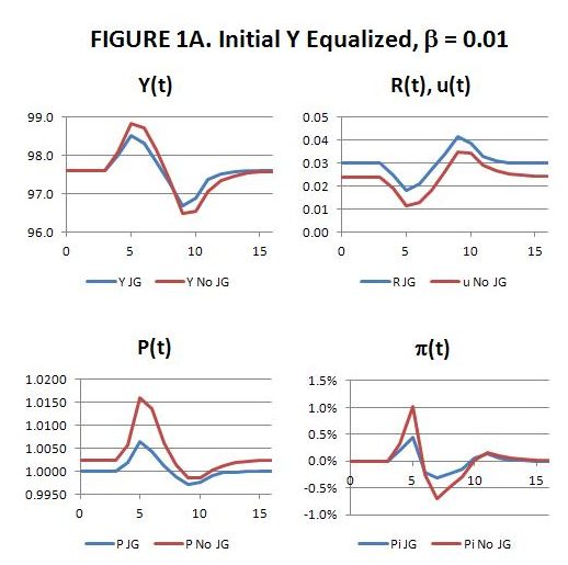
Under the first restriction, both economies start with the same level of output Y = 97.6. Under this restriction, initially A = 48.0 in the JGE model and A = 48.8 in the base model. This restriction causes the price level in the base economy to exceed the price level in the job-guarantee economy at time zero. The reason for this is that the job-guarantee economy can achieve a given output with less sector b employment, due to the contribution of sector j. As a consequence, R < u for any given level of total output Y.
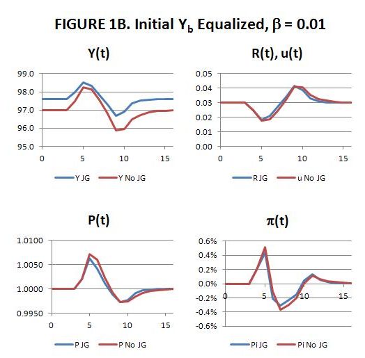
Under the second restriction, the buffer employment ratio in the job-guarantee economy is set equal to the unemployment rate of the base economy (i.e., R = u at first). This requires setting A = 48.0 in the JGE model and A = 48.5 in the base model. This restriction ensures that prices begin at the same level in both economies, but it causes output in the base economy (97.0) to be lower than output in the job-guarantee economy (97.6).
In the present comparison, then, any gains in macroeconomic stabilization achieved through a job guarantee take one of two forms, depending on the restriction applied. Either the job-guarantee economy delivers higher output than the base economy for a similar stability of prices, or it delivers similar output alongside more stable prices.
Two values of β are considered: β = 0.01 and β = 0.05. These values are the same as those selected in part 5 to construct graphs of the short-run relationships between the price level and output, P(Y), and the price level and buffer employment ratio, P(R), that apply in the job-guarantee economy. Accordingly, gaps between P and P0 = 1 in the present illustration correspond to the gaps suggested by the diagrams of part 5.
In the first set of comparisons, β is set to 0.01.

The situation depicted in FIGURE 1A is benign so far as price stability is concerned. With the value of β small, the price level is insensitive to variations in demand. The job guarantee reduces the volatility of output slightly. The gains in price stability are more pronounced, although prices are also quite stable in the base model. Initially R = Rn, whereas u < un, in conformity with the first restriction that output be equalized. The inflation rates, denoted by π, are near zero, especially in the job-guarantee economy.

The scenario shown in FIGURE 1B flows from application of the second restriction. The value of β is once again small. This time there is much less difference in price stability, with the gains from the job guarantee mainly coming from a stronger output performance. Both economies begin with the same degree of slack, with R = Rn and u = un. Even with the stronger output, the job guarantee does deliver slight improvement in price stability, but the difference is negligible. The inflation rates in the two economies are also similar.
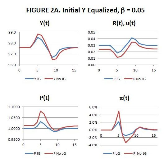
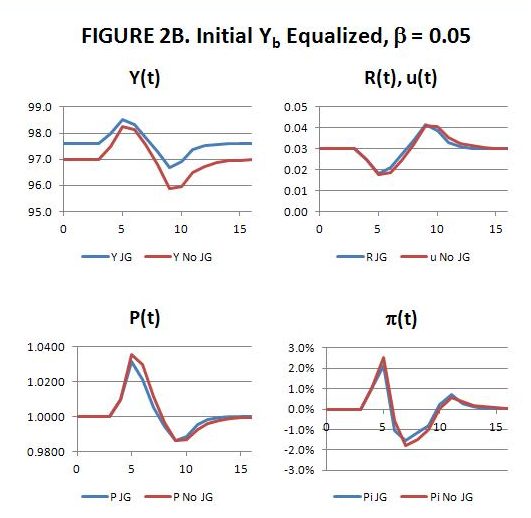
In the second set of comparisons, β is set higher at 0.05. Prices are therefore more sensitive, in these scenarios, to fluctuations in demand and output.

FIGURE 2A shows a marked superiority of the job-guarantee economy in terms of price stability. With β set higher, even modest stabilization of demand and output translates into considerable improvements in price stability when output nears its maximum. Compounding the difference in performance is the effect of the first restriction which, to equalize output initially, requires u < R. Not surprisingly, the job guarantee’s relative gains in price stability and in the curtailment of inflation are most pronounced in this scenario.

When both economies begin with the same degree of slack, as in FIGURE 2B, price behavior and inflation rates are similar. The job guarantee still delivers small gains in price moderation but most of its macro-stabilizing benefits come in the form of stronger activity.
