A Simple Framework for Analyzing a Demand-Led Economy

by
peterc
My articles My booksMy videos
Follow on:Twitter

I have been thinking about a simple depiction of a demand-led economy. Mostly it draws on standard Keynesian macro, Kalecki’s work on cycles and growth, and supermultiplier models developed within the surplus approach. The main focus is on the evolution of a demand-led economy through time. The present post simply sketches the basic framework and provides some context. Perhaps in the future certain aspects can be fleshed out.

 
The Basic Framework

The level of ‘real’ economic activity – as measured in the National Accounts as Gross Domestic Product at constant prices – will be considered demand determined along the lines of Keynes and Kalecki. It is assumed that normally there are reserves of labor-power and other resources as well as spare productive capacity in the form of underutilized plant and equipment. So long as this assumption holds, it is possible for output to be adjusted to demand through variations in the level of activity.

Inside resource and capacity limits, the level of output is regarded as being determined more or less independently of prices. In exceptional circumstances, when demand outstrips the capacity of the economy to respond in real terms, there would be demand-side price pressures and/or non-price rationing. But, for the most part, the economy is considered to be demand constrained, inside ultimate supply-side limits.

This is regarded as true over any time frame. In a period so short that capacity is treated as fixed, output is adjusted to demand through variations in the rate of capacity utilization. In response to stronger demand, firms utilize their given facilities more fully. Over longer time frames, in which capacity should be considered variable, output can be adjusted to demand not only through variations in the utilization rate but by altering capacity itself, investment being the means for doing this.

Both the level of activity and the growth rate of the economy are in this way considered to be demand led.

This perspective on output and growth is intentionally left open in terms of other key economic questions, such as value, price and distribution. This leaves space for competing theories on these matters. If distribution, for instance, is thought to impact systematically on the level of output, it can be introduced through explicit assumptions about the determinants of variables or parameters that, in the present discussion, are simply taken as exogenously given. A well known example is Kalecki’s adoption of the classical assumption that workers, in aggregate, consume all their wages, which makes the size of the multiplier dependent on the distribution between wage and profit income.

The perspective presented here is also open when it comes to the roles of money and finance, although the natural fit with endogenous money and state money theories will probably be evident.

Cumulative developments in the sectoral balances that are thought to impact on private consumption could be worked into an explanation of that part of consumption that here is simply treated as autonomous. Within the framework to be discussed, this would also have an impact on private investment.

 
Keynesian Output Determination

We can start with the standard Keynesian model of output and income determination (although Kalecki’s framework would serve just as well). Total output (Y) is equal to the sum of expenditures. In the simplest versions of the model, all expenditures other than the greater part of private consumption are assumed to be exogenous. Induced consumption is taken to equal c(1 – τ)Y, where c and τ are the marginal propensities to consume and tax, respectively. For simplicity, both are assumed constant. Supposing a closed economy, also for simplicity, exogenous demand includes autonomous private consumption, private investment and government spending. These categories of demand can be grouped together as autonomous expenditure (A). Output will equal the sum of induced consumption and autonomous expenditure:

All variables are taken to be functions of time. Unless there is risk of ambiguity, time subscripts will be omitted. If we let α = 1 – c(1 – τ) represent the marginal propensity to leak to taxes and saving, which implies that c(1 – τ) = 1 – α, the above expression can instead be written as:

This notational choice will simplify some of the algebra later.

If (1) is viewed in terms of actual output, it is merely an identity. The identity holds because of the National Accounting convention of treating changes in inventories, whether anticipated or not, as part of investment. Over time, however, unanticipated variations in inventories can be expected to induce an output response. These inventory changes, to the extent that they are unexpected, amount to unplanned investment. A key assumption of the Keynesian income-expenditure model is that firms expand or cut back production in an attempt to eliminate unplanned investment or disinvestment. Granted this output response to the emergence of excess supply or demand, and given the level of exogenous variables and parameters, there will be a tendency for actual output Y to converge on output level Y* (obtained by solving (1) for Y):

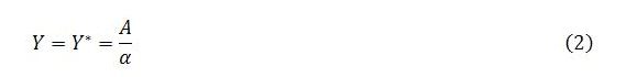
This notional level of output is usually referred to as ‘equilibrium output’. In what follows, it will be the focus of attention. It is possible to delve into the relationship between Y and Y*, but this exercise is left for another day.

The term ‘equilibrium’ is often taken to have quite negative connotations in heterodox circles. With that in mind it is perhaps worth stressing that the requirements of equilibrium, as defined by (2), are far less onerous than those pertaining to some other notions of equilibrium. In particular, there is no implication that all markets must clear. Equilibrium, in the present sense, simply refers to a situation in which planned leakages (in a closed economy, taxes plus saving) happen to equal planned injections (government spending plus private investment) so that the sum of all monetary demand (planned expenditures) equals the sum of output supplied (also measured in monetary terms). There may be mismatches of supply and demand in many markets, but if the excess demands and supplies happen to sum to zero, actual output will be at Y*.

If capacity is taken as fixed – as is often the case in short-run models – Y* will be stable until there is a change in one of the exogenous variables or parameters (summarized as A and α). As will be apparent by the end of the post, over longer time frames, in which capacity is free to vary, neither Y* nor the growth rate of Y* will necessarily be stable other than in the simplest versions of the model that take all expenditure other than induced consumption as exogenous. Over longer time frames, a stable growth rate requires more than an equality of planned leakages and injections. In particular, capacity would need to be fully adjusted to demand.

Importantly, the model does exhibit ‘dynamic stability’ provided that: (i) there is a positive level of autonomous demand (A > 0); and (ii) the marginal propensity to leak is greater than zero (α > 0). The property of dynamic stability is a consequence of the key behavioral assumption that firms seek to eliminate unanticipated changes in inventories. Dynamic stability ensures that there is a continual tendency for Y to converge toward Y*.

The model’s property of dynamic stability perhaps provides some justification for focusing, at least in certain analytical contexts, on the behavior of Y*, rather than explicitly dealing with the distinction between actual and equilibrium output. In what follows, the asterisk in Y* will be dropped unless ambiguity seems likely, with output Y* simply referred to as Y. But it should be kept in mind that discussion pertains to the behavior of notional output Y* rather than actual output Y.

 
A Growing Economy

The growth behavior of this notional level of output, which we are simply denoting Y, can be considered by totally differentiating (1) with respect to time:

Here, Y dot is the derivative of output with respect to time (dY/dt). Similarly, A dot = dA/dt. Collecting terms involving Y dot to the left-hand side gives:

Dividing both sides by αY and multiplying the right-hand side by A/A (= 1) modifies this to:

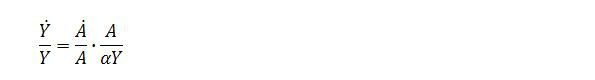
A time derivative of a variable divided by the variable itself gives the variable’s instantaneous growth rate. In our case, Y dot/Y is the instantaneous growth rate of output Y, which can be denoted g. Likewise, A dot/A is the instantaneous growth rate of autonomous spending A, which can be denoted g_A:

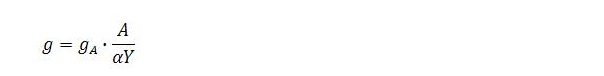
Recalling from (2) that Y = Y* = A / α, the fraction on the right-hand side reduces to one. So, in this simple version of the model, equilibrium output grows at the same rate as autonomous demand:

The growth rate of equilibrium output remains constant so long as the growth rate of autonomous demand remains constant (which, of course, may not be for long at all).

 
A First Complication: Endogenous Private Investment

In terms of growth behavior, the model as presented so far is as simple as it gets. The reason for this is that: (i) all expenditure other than induced private consumption has been assumed exogenous and part of autonomous expenditure; and (ii) the only endogenous component of spending (induced private consumption) has been treated as a constant fraction of income, because of the simplifying assumption that the marginal propensities to consume and tax are both constant. The behavior of equilibrium output becomes a little more complicated once we allow for the idea that private investment is induced by growing output and income. The basic rationale here is that higher rates of capacity utilization, which occur when output is expanded relative to capacity to meet rising demand, will encourage additional investment as a means for firms to adjust capacity to demand.

Following the supermultiplier theory, this situation can be represented by a simple modification of expression (1). Output will now equal the sum of induced consumption, endogenous private investment and autonomous demand:

The second term on the right-hand side, hY, is endogenous planned investment (I = hY). Unlike the marginal propensity to leak, the ‘marginal propensity to invest’ h, while also a fraction between zero and one, is not considered to be a constant. Instead, h is assumed to rise when the rate of capacity utilization is above ‘normal’ and to fall when the utilization rate is below normal. In the present context, the marginal propensity to invest can also be thought of as the investment share in income, because I = hY implies h = I/Y. It is supposed that investment rises and falls as a proportion of income in response to variations in the rate of utilization.

The final term in (1′) is also somewhat altered compared with (1). Z, like A, refers to autonomous expenditure. But this expenditure now also has the characteristic that it does not directly add to private-sector productive capacity. In the literature, this category of expenditure is sometimes referred to as ‘non-capacity-enhancing autonomous demand’. In a closed economy, Z includes autonomous private consumption and government spending. In an open economy, it would also include exports.

Solving (1′) for Y enables us to express equilibrium output as a multiple of autonomous demand Z:

Dynamic stability now requires Z > 0 and α > h. The fraction 1/(α – h) is known as the ‘supermultiplier’. It is larger than the regular multiplier because of the inclusion, in its denominator, of the marginal propensity to invest. (At the same time, compared with (2), a term for investment has been removed from the numerator, so the supermultiplier operates on a level of autonomous expenditure that is smaller than in the simpler version of the model.) For example, if α (the marginal propensity to leak to taxes and saving) is assumed to be 1/2 and, at a given point in time, the marginal propensity to invest happens to be 1/6, the regular expenditure multiplier will be 2 whereas the supermultiplier will be 3. An exogenous increase in Z will cause an expansion of output and income that induces further private consumption and investment.

Differentiating (1′) with respect to time, we have:

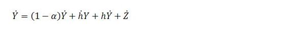
Here, the product rule [d(uv)/dt = u’v + uv’, where u’ and v’ are the time derivatives of u and v, respectively] has been applied to the term hY because both h and Y are functions of time. Collecting all the terms involving Y dot to the left-hand side and factorizing gives:

Following the same basic procedure as earlier, we can divide both sides by (α – h)Y and multiply Z dot by Z/Z to obtain:

Referring back to (2′) we can see that Z/(α – h) = Y, which makes the last fraction in the above expression one. After reordering terms and noting that g = Y dot/Y and g_Z = Z dot/Z, we have:

Growth of equilibrium output now depends not only on the instantaneous growth rate of autonomous demand but also on the instantaneous growth rate of the supermultiplier, which is the second term on the right-hand side of (3′). This last point can be seen by differentiating the supermultiplier 1/(α – h) with respect to time [applying the quotient rule, which says d(u/v)/dt = (u’v – uv’)/v²] and dividing this derivative by the supermultiplier itself. The result is the second term on the right-hand side of (3′).

It is possible to say more about this growth behavior by fleshing out the notion of induced investment, its relationship to the behavior of the utilization rate, and the ongoing attempts by firms to adapt capacity to demand. For now, suffice to note that unless capacity is fully adjusted to demand, h dot (the instantaneous change in the investment share) will be nonzero (other than possibly momentarily when switching sign). As a consequence, equilibrium output will grow more or less rapidly than autonomous demand, according to whether the investment share is rising or falling (h dot is positive or negative). In contrast to the simplest version of the model, the growth rate of equilibrium output is variable rather than constant – even though it pertains to a situation in which supply continually equals demand – unless the investment share has stabilized.

For readers who may be interested, a few earlier posts (for example, here and here) discuss aspects of growth under the assumption of endogenous private investment.

 
Another Complication: A Job Guarantee

It is possible to endogenize other components of spending. Doing so will further modify the growth behavior of equilibrium output. An example that has been touched on in a couple of earlier posts concerns a job guarantee. Under this program, a part of government spending would respond endogenously to variations in output and employment in the broader economy (by which is meant the non-job-guarantee sector). Strictly speaking, this spending would adjust in response to fluctuations in the composition of employment between the two sectors. But it is possible to consider the spending as endogenous with respect to output and income as well, because of the close connection between output and employment.

Modifying expression (1) once more, output for the economy as a whole is now the sum of induced private consumption, endogenous private investment, endogenous job-guarantee spending and autonomous demand:

Here, jY represents government spending on a job guarantee (G_j), where j is the proportion of income spent on the program. Like h, j is variable rather than constant. But unlike h, j varies countercyclically rather than procyclically. It automatically rises in economic downturns and falls during upturns. A couple of earlier posts (here and here) discuss the behavior of job-guarantee spending. In those posts, job-guarantee spending was denoted G_g. From now on, I intend to opt for G_j instead (j for ‘job guarantee sector’) so that g can be reserved for growth rates. Since G_j = jY, it follows that the job-guarantee spending share in income is j = G_j/Y. An expression for j can be derived from the expressions for G_j and Y that are presented in the earlier posts. This is left for a possible future post.

Solving for equilibrium output gives:

Dynamic stability now requires Z > 0 and α – h – j > 0. The supermultiplier has become 1/(α – h – j). An exogenous increase in autonomous demand Z will boost output as well as employment in the broader economy. One consequence is that h will tend to become bigger due to a strengthening of the inducement to invest. Viewed in isolation, this will tend to make the supermultiplier larger. But another consequence of stronger autonomous demand is that j will tend to shrink, because rising output implies a stronger employment outcome in the broader economy, reducing the need for job-guarantee spending. This, viewed in isolation, tends to make the supermultiplier smaller. The overall impact on the supermultiplier will depend on the combined impact of stronger autonomous demand on the investment share (h) and job-guarantee spending share (j).

Adopting the same procedure as we have already adopted twice in earlier sections of the post enables the derivation of an expression for the growth rate of equilibrium output:

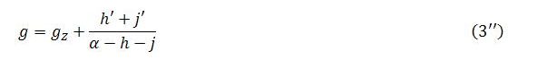
Here, time derivatives are denoted with the prime (‘) symbol rather than dots, because j already has a dot. Expression (3”) says that the growth rate of equilibrium output deviates from the growth rate of autonomous demand to the extent that there are variations in the investment and/or the job-guarantee spending shares in income. As before, the growth rate of equilibrium output will equal the sum of the growth rates of autonomous demand and the supermultiplier.

 
Concluding Remark

Even though we have abstracted from the distinction between actual output Y and equilibrium output Y*, which amounts to assuming that the economy is continuously operating at a level of output that equates aggregate supply with aggregate demand (or planned leakages with planned injections), this does not imply a constant rate of growth (let alone a constant level of output) other than in the simplest versions of the model. In the presence of endogenous investment and/or a job guarantee, stability in the equilibrium growth rate would further require that capacity had fully adjusted to demand (stabilizing the investment share h) and/or the composition of employment had settled at a particular sectoral configuration (stabilizing the job-guarantee-spending share j). Needless to say, there is little reason to expect that such stability in the equilibrium growth rate would ever be maintained for long, or even attained at all.