Disequilibrium Dynamics of Output and Demand

by
peterc
My articles My booksMy videos
Follow on:Twitter

Theoretical studies of output and growth often focus on the behavior of equilibrium output. The usefulness of this approach depends on there being a tendency for actual output to converge on equilibrium output. With such a tendency present, studying the behavior of equilibrium output will tell us something about the behavior of actual output. It is therefore of interest to spell out the process by which an economy in disequilibrium is thought to tend toward equilibrium.

A first step is to consider the disequilibrium behavior of an economy that, for simplicity, is taken to be stationary (non-growing) when in equilibrium. This approach is adopted in the present post. The exercise is really preparation for considering a continually growing economy – a task that is left for a possible future post.

The material in this post is somewhat technical but hopefully not difficult. Even so, the post is long (about 4000 words) and, for readers not already familiar with similar material, possibly a stretch to read all in one go. I considered separating the post into numerous shorter ones but felt that the loss of continuity would require too much repetition in setting up the discussion each time.

The post is divided into sections that provide natural stopping points for readers who wish to take breaks. The section titles are:

1. Macroeconomic Equilibrium
2. Disequilibrium Behavior
3. Adjustment Process
4. Adjustment in Simple Algebra
5. Convergence as a Power Series: λ = 1
6. Convergence as a Power Series: λ < 1
7. Adjustment of Growth Rates

Some background information relating to 1 can be found in the ‘Short & Simple’ series (mainly here). A very helpful reference for some of the material covered in later sections is Ronald Shone’s book, An Introduction to Economic Dynamics, Cambridge University Press. The edition I have was published in 2003. In particular, the third chapter provides more sophisticated – but still highly accessible – treatments of 3 and 4. The purpose of 7 is to lay some groundwork for a possible future post on a continually growing economy.

 
1. Macroeconomic Equilibrium

The notion of macroeconomic equilibrium relates to plans (or desires). Although, under National Accounting conventions, actual output equals actual expenditure by definition, equilibrium will only occur if actual output equals planned expenditure.

The sum of planned expenditures constitutes total demand. Actual output represents total supply. Accordingly, the equality of demand and supply requires that actual output and actual expenditure equal planned expenditure. This only occurs when unplanned expenditure is zero.

Unplanned expenditure is possible because of the way actual expenditure is defined. Included in actual expenditure is the change in inventories, meaning the change in unsold stocks of goods held by firms. The change in inventories is treated, in the National Accounts, as expenditure by firms to themselves.

From a theoretical standpoint, intended changes in inventories are part of planned investment. Unintended changes in inventories amount to unplanned investment.

Defined in this way, unplanned investment is identically equal to excess supply. It is the amount of output that firms intended to sell but were unable to sell within the period. In other words, unplanned investment is the excess of supply over demand.

In symbols:

Here, I_u is unplanned investment (the unanticipated change in inventories). Y is actual output (supply). Y_d is planned expenditure (demand).

Equilibrium occurs if unplanned investment is zero (I_u = 0) so that:

where Y* is the equilibrium level of output.

Total planned expenditure (Y_d) can be grouped into two broad categories. ‘Autonomous demand’ (A) is considered exogenous and independent of income. It includes the planned exogenous spending of households, firms, government and foreigners and is defined net of exogenous imports. ‘Induced demand’ is endogenous and depends on income. It is defined net of endogenous imports. In general, endogenous spending can be undertaken by households, firms or government. But to keep the present discussion as simple as possible, all expenditure other than net induced consumption (defined as induced consumption minus endogenous imports) will be considered exogenous and part of A. If the marginal propensity to leak to taxes, saving and imports is denoted by α – assumed to be a constant fraction between zero and one – there will be induced demand of (1 – α)Y.

Total demand, then, is the sum of the induced and autonomous components of planned expenditure:

Actual output, which is identically equal to actual expenditure, includes not only planned expenditure but also unplanned investment:

When unplanned investment is zero, actual output (Y) equals planned expenditure (Y_d) and is at the equilibrium level (Y*). Substituting the expression for Y_d in (3) into equilibrium condition (2) gives:

Solving for Y:

Since both autonomous demand (A) and the marginal propensity to leak (α) are taken as given, equilibrium output (Y*) is stable unless there is an exogenous change in A or α.

Although, for given A and α, Y* is stable, actual output (Y) and planned expenditure (Y_d) only equal Y* in equilibrium. Our present concern is with what happens out of equilibrium.

 
2. Disequilibrium Behavior

In the income-expenditure model, it is assumed that firms respond to unexpected changes in inventories (excess demand or supply) by varying levels of production. The model is valid provided there is sufficient spare capacity, underutilized labor-power and resources for firms to respond in this way.

In a situation of excess supply, unwanted inventories mount (I_u > 0) and firms are assumed to cut back production. This initiates a multiplier process that causes actual output (and to a lesser extent demand, through the effects on induced demand) to decline toward the equilibrium level.

Conversely, when there is excess demand, firms are assumed to step up production in an attempt to replenish dwindling inventories. This sets off a multiplier process in which actual output (and to a lesser extent demand) rise toward the equilibrium level.

So, in a situation of excess demand:

An expansion of production will induce consumption and cause both actual output and planned expenditure to rise toward the equilibrium level of output.

In a situation of excess supply:

and the reverse process occurs.

 
3. Adjustment Process

Suppose the economy is initially out of equilibrium. We can consider the process of adjustment.

Throughout the exercise, both autonomous demand (A) and the marginal propensity to leak (α) will be held constant. This means that the equilibrium level of output (Y*) will also remain constant throughout the adjustment process as actual output and planned expenditure converge on Y* = A_/α.

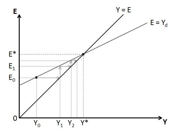
A well known diagram is often used to illustrate the situation. It is shown below. In the diagram, expenditure (E) is measured along the vertical axis. Output and income (Y) are measured along the horizontal axis.

The level of planned expenditure associated with each level of output is indicated by the Y_d schedule. At points off this schedule, actual expenditure differs from planned expenditure by an amount corresponding to unplanned investment.

The 45-degree line shows all the points at which actual output equals actual expenditure; that is, all the points at which Y = E.

As has already been established, equilibrium requires that planned expenditure (Y_d) equals actual output (Y). This occurs at the point of intersection between the Y_d schedule and the 45-degree line. Since actual output equals actual expenditure by definition, the point of intersection also represents a situation in which planned expenditure equals actual expenditure.

All points on the Y_d schedule to the left of the 45-degree line show situations of excess demand (Y_d > Y), whereas points on the Y_d schedule to the right of the 45-degree line indicate excess supply (Y > Y_d).

Suppose initially that actual output is at the level Y₀. This is a situation of excess demand. Planned expenditure E₀ exceeds actual output Y₀.

The difference between demand and supply, which defines unplanned investment, is represented by the horizontal distance from output Y₀ to output Y₁. It is also measured by the vertical distance between the Y_d schedule and the 45-degree line at output Y₀.

In the present situation, unplanned investment is negative because demand exceeds supply (Y_d > Y).

Although only output of Y₀ is actually produced in period zero (denoted t = 0), firms are able to satisfy demand of E₀ by running down inventories.

The unexpected depletion of inventories acts as a signal for firms to expand production in the next period (t = 1) to the level of output Y₁.

The diagram is drawn on a simplifying assumption that firms make the full adjustment from Y₀ to Y₁ in a single period. In general, they might only make part of this adjustment within the period. (They might even make more than the full adjustment, but this possibility will be ignored in the present discussion.) The basic logic of the model is not affected by the strength of reaction to excess demand or supply, but the convergence process will take a bit longer in the case of partial adjustment.

Even the full adjustment from Y₀ to Y₁ does not immediately result in equilibrium, because the additional income (ΔY = Y₁ – Y₀) induces extra private consumption. This is represented as a movement up along the Y_d schedule.

So, at output Y₁, planned expenditure is still greater than actual output. This can be seen by the fact that, at output Y₁, the Y_d schedule is still above the 45-degree line.

Importantly, though, there is less excess demand at time t = 1 than at time t = 0. The reason for this is that the slope of the Y_d schedule is flatter than the 45-degree line. Demand rises more gradually than supply as both increase toward the equilibrium level of output.

Specifically, the Y_d schedule’s slope is less than one. (Its slope is 1 – α, which is less than 1 because α > 0.) In contrast, the slope of the 45-degree line is equal to 1. The difference in slopes makes it possible for supply to catch up to demand as firms attempt to adjust actual output to demand.

Within the model, the relative flatness of the Y_d schedule is actually one of two conditions that, when satisfied, ensure convergence of actual to equilibrium output, or what is called ‘dynamic stability’.

Both conditions for dynamic stability relate to the Y_d schedule and are depicted in the diagram. They are that:

(i) there is a positive level of autonomous demand (A > 0), which means that the Y_d schedule must have a positive vertical intercept; and

(ii) the marginal propensity to leak is positive (α > 0), which means that the slope of the Y_d schedule (1 – α) must be less than one.

The first condition – a positive vertical intercept – ensures that if the Y_d schedule crosses the 45-degree line at an equilibrium point, it will do so at a positive level of output. This is important because only positive levels of output make economic sense.

The second condition – a positive marginal propensity to leak – ensures that the two schedules will cross, because it means the Y_d schedule is flatter than the 45-degree line.

Provided the conditions for dynamic stability are satisfied, the convergence process will eventually cause output to reach (asymptotically) the level Y*, where supply equals demand (Y = Y_d = Y*).

The process is indicated by the arrows. Each time firms respond to a deficiency of inventories by stepping up production, this induces extra demand, but not as much demand as the additional income that has been created, because of a positive marginal propensity to leak from the circular flow of income.

A similar process would occur from a position of excess supply at which the point on the Y_d schedule happened to be to the right of the 45-degree line. There would be a multiplied decline in actual output as each contraction in the level of production shrunk induced demand, but not by as much as the reduction in income.

 
4. Adjustment in Simple Algebra

The adjustment process just described can be expressed in simple algebra.

Recall, from (1), that unplanned investment is identically equal to the amount of excess supply in the economy:

It has been assumed that, out of equilibrium, firms attempt to eliminate part or all of the unplanned investment in the next period. This suggests that, in the next period, firms will adjust production by the amount

where λ is a positive fraction. The minus sign in (7) indicates that firms adjust actual output in the opposite direction to the change in unplanned investment. For example, if demand is 990 and actual output only 980, implying unplanned investment of -10, it is assumed that output in the next period will be increased by some fraction (λ) of 10.

The expression for unplanned investment in (1) can be substituted into (7):

This says that the change in actual output (ΔY) can be expressed as a fraction (λ) of excess demand (Y_d – Y).

From (3), we know that Y_d = (1 – α)Y + A. Substituting for Y_d in (8) and rearranging gives:

This expression makes it possible to work out actual output for the next period as the sum of current-period output and next period’s change in output (Y + ΔY). To do so, we can add Y to both sides of (9) and rearrange:

If we are considering periods t and t+1, this can instead be written:

This is a recursive equation. We can repeatedly substitute the value of actual output in one period (Y_t) to obtain actual output of the following period (Y_t+1).

For example, suppose in period t = 0 that autonomous demand is 500, with the marginal propensity to leak a constant 0.5. The equilibrium level of output will be Y* = A_{/α = 1000. But perhaps firms have only produced actual output of 980 in the period.}

According to the behavioral assumption, firms will increase production each period until equilibrium is restored. In the simplest case of full adjustments (λ = 1), actual output in successive periods will be:

The squiggly equals sign in the final row says that Y_n is ‘asymptotically equal’ to the equilibrium value. That is, actual output approaches the equilibrium level asymptotically.

The logic of the adjustment process just outlined can also be considered in a slightly different way by assuming, as an alternative exercise, that the economy is initially in equilibrium and then working through the effect of a one-off exogenous change in autonomous demand.

Suppose A = 490, α = 0.5, and the economy is initially in equilibrium with both actual output and total demand equal to 980. If autonomous demand then increases by 10 to 500 (giving ΔA = 10), this will result in excess demand and call for an expansion of production by firms. If we take the change in autonomous demand to have occurred in “period 0”, then the disequilibrium adjustment process will be an exact replica of the one shown above.

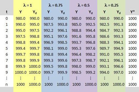
If λ happens to be less than 1, the adjustment will be more gradual. The following table, which continues with the same example, shows the sequence of actual output and total demand for various values of λ. Total demand is calculated each step by substituting the most recent value for actual output into (3), which says that Y_d = (1 – α)Y + A.

In the table, autonomous demand is held constant at A = 500, the marginal propensity to leak is α = 0.5 and a situation of excess demand is assumed to exist in period 0.

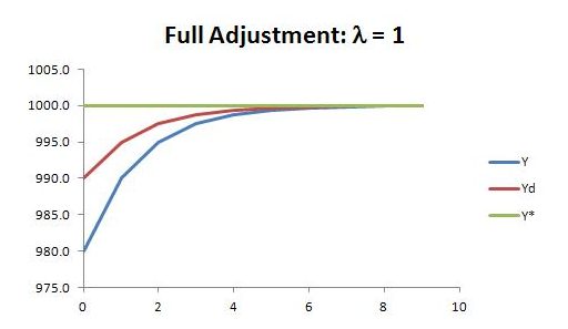
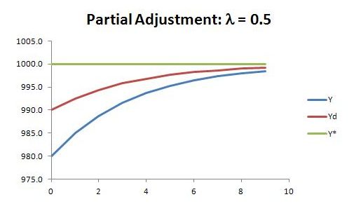
Here are a couple of cases represented in graphical form:

 
5. Convergence as a Power Series: λ = 1

We have observed that actual output and demand both tend to converge to a level that is a multiple of autonomous demand. In equilibrium, Y = Y_d = Y* = A_/α.

As is well known, the expenditure multiplier (1_{/α) can be interpreted as the sum of a power series:}

When α takes a value between zero and one, which is always the case under the assumptions of the income-expenditure model, the above series asymptotically approaches 1_{/α as n becomes large.}

The power series can be interpreted as tracing out each step of the adjustment process in which actual output adjusts to its equilibrium level.

Starting from a position of equilibrium, reconsider the consequences of a one-off exogenous change in autonomous demand, denoted ΔA.

The change in autonomous demand will cause a multiplied change in equilibrium output of:

Here, the sum of the power series given in (11) has been substituted for the multiplier 1_/α.

Continuing with the example, if actual and equilibrium output were initially 980, the marginal propensity to leak 0.5 and the change in autonomous demand 10, then equilibrium output would eventually increase by 20. Applying (12), with α = 0.5 and ΔA = 10:

If it is assumed that firms make a full adjustment each period (meaning λ = 1), then each step in the convergence process toward equilibrium will correspond to one of the terms in the infinite series shown above.

The initial change in autonomous demand (ΔA = 10) causes a situation of excess demand. Actual output is 980, whereas total planned expenditure has suddenly increased to 990. Firms meet the higher demand by running down inventories by 10. This represents unplanned investment of -10.

By assumption, firms respond by trying to eliminate the unplanned investment. In step 0 of the adjustment (t = 0), firms expand production by 10. This is equal to the first term in the power series: 10 x 1 = 10(1 – 0.5)⁰.

The increase in actual output of 10 induces extra expenditure of 5, equal to (1 – α)ΔY. As a result, there is still excess demand, but now only of 5 rather than 10.

In step 1 (t = 1), firms expand production again, this time by 5. This corresponds to the second term in the power series: 10(0.5) = 10(1 – 0.5)¹.

More generally, the adjustment that firms make in step t of the convergence process will be given by the tth term in the series: ΔA(1 – α)^t = 10(1 – 0.5)^t. For instance, in step 3, firms adjust output by 10(1 – 0.5)³ = 1.25.

The sum of the adjustments made over n steps asymptotically approaches 20, with both actual output and planned expenditure converging on 1000.

Visually, this adjustment has already been illustrated in the graph provided earlier for the case of λ = 1.

 
6. Convergence as a Power Series: λ < 1

We have seen that if λ takes a value less than 1, the adjustment process will be more gradual. The power series needs to be modified to:

This is a more general version of (12). In the special case of λ = 1, the above formula reduces to the earlier one. The effect of λ < 1 is to spread the adjustment process over more steps. The adjustment in the initial step is smaller, but the size of the adjustment each period shrinks less rapidly than when λ = 1.

The value of λ affects the speed of adjustment but, within the model, not the level to which actual output and demand converge. Since Y* = A_{/α, the point of convergence depends only on autonomous demand (A) and the marginal propensity to leak (α).}

The rest of this section can be skipped without missing much economic content. But for readers who may be curious, it is pretty easy to arrive at the formula given in (12′). Each step of the adjustment process can be described algebraically, beginning with t = 0, until a clear pattern emerges. Since this kind of scenario arises quite frequently in economics, perhaps it is worth spelling out the working.

The sequence of events begins with a one-off change in autonomous demand, or ΔA. This creates excess demand of ED₀ = ΔA. In response, firms begin to adjust actual output to demand by trying to eliminate unplanned investment.

Let Δ_tY be the change in actual output at step t of the adjustment process. The change in actual output (and income) will induce additional private consumption (net of endogenous imports) of Δ_tC. Specifically, a fraction (1 – α) of the extra income will go to induced demand. This constitutes excess demand, but less than was created in earlier steps.

The excess demand of period t (ED_t) will be reduced in period t+1 to the extent that extra output is produced in the new period, but will be increased to the extent that extra demand is induced. That is, ED_t+1 = ED_t – Δ_tY + Δ_tC.

Putting all this together, a pattern emerges within a few steps:

The adjustment of actual output in step t will be equal to λΔA(1 – αλ)^t. When t = 0, this reduces to λΔA. When t = 1, the expression reduces to λΔA(1 – αλ).

The total change in actual output over the entire adjustment process will be the sum of all these step adjustments, which is what (12′) says.

 
7. Adjustment of Growth Rates

It is also possible to represent the adjustment process in terms of growth rates. This will be useful if considering an economy with a continual tendency to grow over time (a task left for another time).

At the moment, we are considering a simpler economy that only grows (or shrinks) in the process of adjustment to equilibrium. So, in the present context, the growth rate will settle at zero once equilibrium is reached.

Recall that unplanned investment, as defined earlier in (1), is identically equal to the amount of excess supply in the economy:

We have expressed the change in actual output as a function of excess demand. Combining (7) and (8) from earlier:

If, conceptually, we break down the steps of the adjustment process into tiny enough increments of time, we can think of the adjustment process as a continuous one and recast (8) as:

Here, Y dot is the derivative of output with respect to time (dY_/dt).

The growth rate of actual output (g) is found by dividing Y dot by Y:

This growth rate diverges from zero whenever the economy is out of equilibrium. In situations of excess demand, Y_d /_{Y is greater than one and the actual growth rate rises above zero. The growth rate will remain positive until equilibrium (Yd /Y = 1) is attained. Conversely, the actual growth rate is negative in situations of excess supply, and remains that way until convergence is complete.}

Under present assumptions, the equilibrium growth rate (g*) is determined by the exogenously given growth rate of autonomous demand. This can be seen by differentiating the expression for equilibrium output (Y* = A_{/α) with respect to time and dividing by Y*:}

Since autonomous demand is being held constant throughout the adjustment process, g_A and g* are both zero over the relevant time horizon.

In more elaborate versions of the model, the behavior of the equilibrium growth rate can be more complicated. The simplicity, in the present context, is due to: (i) all demand other than net induced consumption being treated as exogenous; and (ii) the marginal propensity to leak being assumed strictly constant. Introducing more endogenous elements to demand will complicate the behavior of g*. (Examples involving endogenous investment and an endogenous component to government spending are discussed in a previous post.)

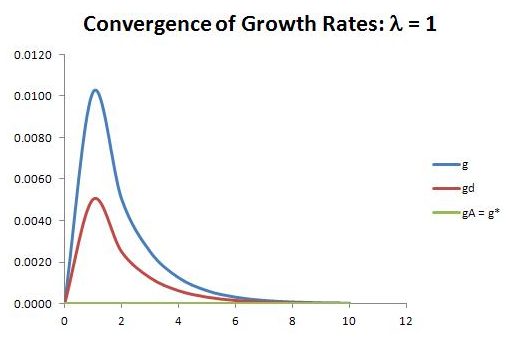
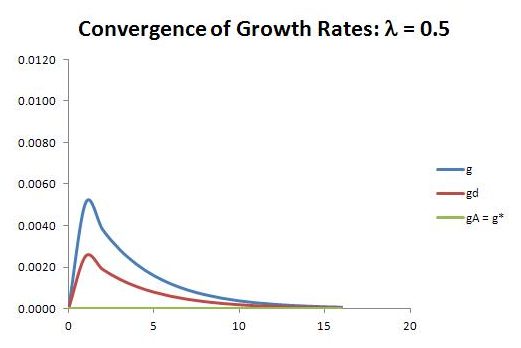
The convergence of the actual growth rate (g) to the equilibrium growth rate g* (and g_A) is illustrated below for a couple of values of λ.

The growth behavior of total demand is also illustrated in these diagrams. Like actual output, demand grows at a rate other than zero outside equilibrium. Its growth rate (g_d) does not diverge as far from the equilibrium growth rate as g does, because the required adjustment of demand is less than the required adjustment of output. By the logic of the model, whenever there is disequilibrium, production needs to “catch up” to demand. To do so, it needs to grow (or shrink) faster than demand during the process of adjustment.

The growth behavior of demand is implicit in (3), which defines planned expenditure as the sum of induced and autonomous demand:

Differentiating this expression with respect to time gives:

Dividing through by Y_d and multiplying Y dot by Y_{/Y and A dot by A/A gives:}

The expression for g in (13) can now be substituted into the growth equation for demand. Upon rearrangement:

Since the level of autonomous demand is held constant throughout the adjustment process, the growth rate of autonomous demand (g_A) is zero, making the second term on the right-hand side of (14) also zero:

The sign of g_d simply depends on whether the fraction Y_{/Yd is greater than, equal to, or less than one. When there is excess demand, Y/Yd is less than one and gd is positive. This is consistent with the behavior depicted in the diagrams above. In the reverse case of excess supply, Y/Yd is greater than one and gd is negative. In equilibrium, the term on the right-hand side of (14′) vanishes and gd equals zero, as expected.}

It has been stated that, out of equilibrium, the divergence of g from the equilibrium growth rate (g* = g_A = 0) is greater than the divergence of g_d. This can be verified working from the expressions for g and g_d provided by (13) and (14′), respectively:

The growth rate of actual output (g) will be greater in absolute value than the growth rate of total demand (g_d) provided:

From (4), Y = (1 – α)Y + A + I_u, which implies that I_u = αY – A. This can be substituted for I_u in the above inequality to obtain the following condition:

This is one of the two conditions for dynamic stability already discussed. Since, within the model, there is always a positive amount of autonomous demand, the condition A > 0 automatically holds. This verifies that, out of equilibrium, the absolute value of g will exceed the absolute value of g_d. In other words, g will take more extreme values than g_d during convergence to equilibrium.

It is possible to say more about the growth behavior of actual output, total demand and equilibrium output, but this is perhaps better left for a discussion of a continually growing economy.