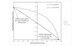
Figure 1: A Wage Frontier With Two Fluke Switch Points This post presents an example with circulating capital alone. Table 1 presents the technology for an economy in which two commodities, iron and corn, are produced. One process is known for producing iron, and two are known for producing corn. Each process is specified by coefficients of production, that is, the required inputs per unit output. The Alpha technique consists of the iron-producing process and the first corn-producing process. Similarly, the Beta technique consists of the iron-producing process and the second corn-producing process. At any time, managers of firms face a problem of the choice of technique. Table 1: The Coefficients of Production InputIron IndustryCorn IndustryAlphaBetaLabora0,1 = 1a0,2α = 0.7174 e-σ ta0,2β
Topics:
Robert Vienneau considers the following as important: Example in Mathematical Economics, Labor Markets, Sraffa Effects
This could be interesting, too:
Robert Vienneau writes Austrian Capital Theory And Triple-Switching In The Corn-Tractor Model
Robert Vienneau writes Double Fluke Cases For Triple-Switching In The Corn-Tractor Model
Robert Vienneau writes The Emergence of Triple Switching and the Rarity of Reswitching Explained
Robert Vienneau writes Recap For A Triple -Switching Example
| Figure 1: A Wage Frontier With Two Fluke Switch Points |
This post presents an example with circulating capital alone. Table 1 presents the technology for an economy in which two commodities, iron and corn, are produced. One process is known for producing iron, and two are known for producing corn. Each process is specified by coefficients of production, that is, the required inputs per unit output. The Alpha technique consists of the iron-producing process and the first corn-producing process. Similarly, the Beta technique consists of the iron-producing process and the second corn-producing process. At any time, managers of firms face a problem of the choice of technique.
| Input | Iron Industry | Corn Industry | |
| Alpha | Beta | ||
| Labor | a0,1 = 1 | a0,2α = 0.7174 e-σ t | a0,2β = 1.282 e-φ t |
| Iron | a1,1 = 9/20 | a1,2α = 0.001764 e-σ t | a1,2β = 0.3375 e-φ t |
| Corn | a2,1 = 2 | a2,2α = 0.5386 e-σ t | a2,2β = 0.135 e-φ t |
Technical progress, as in structural economic dynamics (Pasinetti 1981), results in decreasing coefficients of production. The coefficients in each corn-producing process decrease at the same rate, but vary between the processes. With wages paid out of the surplus product at the end of the period of production, the wage curves for the two techniques are depicted in Figure 1 for a particular parametrization of the coefficients of production. At this moment in time, the Beta technique is cost-minimizing for any feasible distribution of income. If the wage is zero and the workers live on air, the Alpha technique is also cost-minimizing.
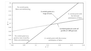
A switch point is defined in this model to be an intersection of the wage curves. These switch points are fluke cases in that almost any variation in the model parameters destroys their interesting properties. A switch point exists at a rate of profits of -100 percent only along a knife edge in the parameter space (Figure 2). Likewise, a switch point exists on the axis for the rate of profits only along another knife edge. The illustrated example, with two fluke switch arises at a single point in the parameter space, where these two partitions intersect.
| Figure 2: The Parameters Space for the Reverse Substitution of Labor |
Figure 2 depicts a partition of the parameter space around the point with these two fluke switch points. Above the more steeply-sloping locus, the switch point on the axis for the rate of profits has disappeared below the axis. The Beta technique is cost-minimizing for all feasible non-negative rates of profits. Below this locus, the Alpha technique is cost-minimizing for a low enough wage or a high enough feasible rate of profits.
In the north east, the switch point at a negative rate of profits occurs at a rate of profits lower than 100 percent. Around the switch point at a positive rate of profits, a lower wage is associated with a corn-producing process with the larger coefficient for labor. That is, a0,2α(σ t) > a0,2β(φ t).
In the south east of Figure 2, the switch point for a positive rate of profits exhibits the reverse substitution of labor. Around this switch point, a lower wage is associated with the adoption of a process producing the consumer good in which less labor is employed per unit of gross output. The other switch point exists for a rate of profits between -100 percent and zero. Steedman (2006) presents examples with this phenomenon in models with other structures.
Qualitative changes in the wage frontier exist in the parameter space away from the part graphed in Figure 2. The analysis presented here is only local to the depicted fluke case.
 Heterodox


