Figure 1: Variation of the Technique with Markup in Agriculture This post is a continuation a of a previous example. I suppose this is the first example in post Sraffian price theory which combines intensive rent and markup pricing. I do not plan on trying to publish it, in a stand-alone article. D'Agata (1983) sets some coefficients to zero to simplify it for his purposes. I would like a range of parameters where I get reswitching or capital-reversing. I have found a case where, given the wage, the cost-minimizing technique is not unique away from switch points. I would like an example where some of the locii in Figure 2 below intersect. I might as well repeat the data. Table 1 shows the coefficients of production. Only one type of land exists, and three processes are known for
Topics:
Robert Vienneau considers the following as important: Full Cost Prices, rent
This could be interesting, too:
Robert Vienneau writes Variations In An Analysis Of Intensive Rent With One Type Of Land (Part 2/2)
Robert Vienneau writes Variations In An Analysis Of Intensive Rent With One Type Of Land (Part 1/2)
Robert Vienneau writes Intensive Rent With Two Types Of Land
Robert Vienneau writes Intensive Rent And The Order Of Rentability
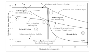
| Figure 1: Variation of the Technique with Markup in Agriculture |
This post is a continuation a of a previous example.
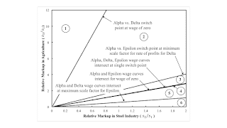
I suppose this is the first example in post Sraffian price theory which combines intensive rent and markup pricing. I do not plan on trying to publish it, in a stand-alone article. D'Agata (1983) sets some coefficients to zero to simplify it for his purposes. I would like a range of parameters where I get reswitching or capital-reversing. I have found a case where, given the wage, the cost-minimizing technique is not unique away from switch points. I would like an example where some of the locii in Figure 2 below intersect.
I might as well repeat the data. Table 1 shows the coefficients of production. Only one type of land exists, and three processes are known for producing corn on it. Following D'Agata, assume that one hundred acres of land are available and that net output consists of 90 tons iron, 60 tons steel, and 19 bushels corn. The net output is also the numeraire.
| Input | Industry | ||||
| Iron | Steel | Corn | |||
| I | II | III | IV | V | |
| Labor | 1 | 1 | 1 | 11/5 | 1 |
| Land | 0 | 0 | 1 | 1 | 1 |
| Iron | 0 | 0 | 1/10 | 1/10 | 1/10 |
| Steel | 0 | 0 | 2/5 | 1/10 | 1/10 |
| Corn | 1/10 | 3/5 | 1/10 | 3/10 | 2/5 |
All three commodities must be produced for any composition of net output. Table 2 lists the available techniques. Only Alpha, Delta, and Epsilon are feasible for these requirements for use. Not all land is farmed and only one corn-producing process is operated under Alpha. Two corn-producing processes are operated together under Delta and Epsilon.
| Technique | Processes |
| Alpha | I, II, III |
| Beta | I, II, IV |
| Gamma | I, II, V |
| Delta | I, II, III, IV |
| Epsilon | I, II, III, V |
| Zeta | I, II, IV, V |
In the non-competitive case, the relative markups in different industries are taken as given. Let the rates of profits be in proportions of s1, s2, and s3, respectively.
Figure 1, at the top of the post, shows the variation in the analysis of the cost-minimizing technique with perturbations of the markup up in agriculture. In drawing this figure, markups in iron and corn production, s1 and s2, are assumed unity. At the intersection between the Alpha and Delta wage curves, the rent for Delta is zero. The scale factor at this switch point is the maximum for the Delta technique. At a switch point between Alpha and Epsilon in regions 1, 2, 3, and 4, the rent for epsilon is zero. The scale factor at such a switch point is the maximum scale factor for Epsilon. In regions 5 and 6, the maximum scale factor for Epsilon is the scale factor for which the wage turns negative.
A fluke case exists off to the right where the wage curves for Alpha at Delta intersect at the maximum scale factor for the rate of profits for Alpha. At that switch point, Delta has a scale factor for the rate of profits of zero percent and a rent of zero. The fluke case partitioning regions 2 and 3 is one where the wage curves for Alpha and Epsilon intersect at the scale factor where the wage for Delta first turns positive. The fluke case partitioning regions 3 and 4 is one in which the wage curves for Alpha, Delta, and Epsilon all intersect at a single switch point.
The fluke cases partition regions 4 & 5 and 5 & 6 change some characteristics of the range of the scale factor of the rate of profits in which no cost-minimizing technique exists. At the fluke case partitioning regions 4 and 5, the wage curves for Alpha and Epsilon intersect at the maximum scale factor for Alpha. I have previously provided an analysis of the fluke case dividing regions 5 and 6. Maybe I should not consider these two fluke cases since they arise, in some sense, for switch points off the frontier.
Anyways, Table 2 shows how the analysis of the choice of technique varies among the numbered regions. If wants to look at these results in some detail, one can relate the variation in the analysis of the choice of technique to the fluke cases.
| Region | Range for Scale Factor | Cost-Minimizing Techniques |
| 1 | 0 ≤ r ≤ R*,ε | Epsilon |
| R*,ε ≤ r ≤ Rα | Alpha | |
| 2 | 0 ≤ r ≤ R*,ε | Epsilon |
| R*,ε ≤ r ≤ Rδ | Alpha | |
| Rδ ≤ r ≤ R*,δ | Alpha and Delta | |
| R*,δ ≤ r < Rα | None. Wage for Alpha positive. | |
| 3 | 0 ≤ r ≤ Rδ | Epsilon |
| Rδ ≤ r ≤ R*,ε | Delta and Epsilon | |
| R*,ε ≤ r ≤ R*,δ | Alpha and Delta | |
| R*,δ ≤ r < Rα | None. Wage for Alpha positive. | |
| 4 | 0 ≤ r ≤ Rδ | Epsilon |
| Rδ ≤ r ≤ r* | Delta and Epsilon | |
| r* ≤ r ≤ R*,δ | None. Wage for Alpha, Delta, Epsilon positive. Rent for Delta and Epsilon positive. | |
| R*,δ ≤ r < R*,ε | None. Wage for Alpha and Epsilon positive. Rent for Epsilon positive. | |
| R*,ε ≤ r < Rα | None. Wage for Alpha positive. | |
| 5 | 0 ≤ r ≤ Rδ | Epsilon |
| Rδ ≤ r ≤ r* | Delta and Epsilon | |
| r* ≤ r ≤ R*,δ | None. Wage for Alpha, Delta, Epsilon positive. Rent for Delta and Epsilon positive. | |
| R*,δ ≤ r ≤ Rε | None. Wage for Alpha, Epsilon positive. Rent for Epsilon positive. | |
| Rε ≤ r < Rα | None. Wage for Alpha positive. | |
| 6 | 0 ≤ r ≤ Rδ | Epsilon |
| Rδ ≤ r ≤ r* | Delta and Epsilon | |
| r* ≤ r ≤ Rε | None. Wage for Alpha, Delta, Epsilon positive. Rent for Delta and Epsilon positive. | |
| Rε ≤ r ≤ R*,δ | None. Wage for Alpha, Delta, positive. Rent for Delta positive. | |
| R*,δ ≤ r < Rα | None. Wage for Alpha positive. |
Figure 2, for completeness, illustrates the partition of the parameter space of markups, where the ratios of markups in iron and steel need not be the same. Figure 1 illustrates what happens along a vertical line in Figure 2 at s2/s1 is unity. I realize it is hard to see region 4 and to distinguish its boundaries in Figure 2.
| Figure 2: Partition Of Parameter Space |
I do not draw any great conclusions. This example demonstrates my visualization techniques and perturbation analysis can be applied to an example where the cost-mninimizing technique is not found from a frontier of wage curves. The non-uniqueness and non-existence of a cost-minimizing technique arises in D'Agata's original example.
 Heterodox


