(Dan here…lifted and reposted) by Mike Kimel How Keynesian Policy Led Economic Growth In the New Deal Era: Three Simple Graphs November 22, 2011 In this post, I will show that during the New Deal era, changes in the real economic growth rate can be explained almost entirely by the earlier changes in federal government’s non-defense spending. There are going to be a lot of words at first – but if you’re the impatient type, feel free to jump ahead to the graphs. There are three of them. The story I’m going to tell is a very Keynesian story. In broad strokes, when the Great Depression began in 1929, aggregate demand dropped a lot. People stopped buying things leading companies to reduce production and stop hiring, which in turn reduced how much people could buy
Topics:
Dan Crawford considers the following as important: Healthcare, politics, Taxes/regulation, US/Global Economics
This could be interesting, too:
Robert Skidelsky writes Lord Skidelsky to ask His Majesty’s Government what is their policy with regard to the Ukraine war following the new policy of the government of the United States of America.
Joel Eissenberg writes No Invading Allies Act
Ken Melvin writes A Developed Taste
Bill Haskell writes The North American Automobile Industry Waits for Trump and the Gov. to Act
(Dan here…lifted and reposted)
by Mike Kimel
How Keynesian Policy Led Economic Growth In the New Deal Era: Three Simple Graphs
November 22, 2011
In this post, I will show that during the New Deal era, changes in the real economic growth rate can be explained almost entirely by the earlier changes in federal government’s non-defense spending. There are going to be a lot of words at first – but if you’re the impatient type, feel free to jump ahead to the graphs. There are three of them.
The story I’m going to tell is a very Keynesian story. In broad strokes, when the Great Depression began in 1929, aggregate demand dropped a lot. People stopped buying things leading companies to reduce production and stop hiring, which in turn reduced how much people could buy and so on and so forth in a vicious cycle. Keynes’ approach, and one that FDR bought into, was that somebody had to step in and start buying stuff, and if nobody else would do it, the government would.
So an increase in this federal government spending would lead to an increase in economic growth. Even a relatively small boost in government spending, in theory, could have a big consequences through the multiplier effect – the government hires some construction companies to build a road, those companies in turn purchase material from third parties and hire people, and in the end, if the government spent X, that could lead to an effect on the economy exceeding X.
This increased spending by the Federal government typically came in the form of roads and dams, the CCC and the WPA and the Tennessee Valley Authority, in the Bureau of Economic Analysis’ National Income and Product Accounts (NIPA) tables it falls under the category of nondefense federal spending.
Now, in a time and place like the US in the early 1930s, it could take a while for such nondefense spending by the federal government to work its way through the economy. Commerce moved more slowly back in the day. It was more difficult to spend money at the time than it is now, particularly if you were employed on building a road or a dam out in the boondocks. You might be able to spend some of your earnings at a company store, but presumably the bulk of what you made wouldn’t get spent until you get somewhere close to civilization again.
So let’s make a simple assumption – let’s say that according to this Keynesian theory we’re looking at, growth in any given year a function of nondefense spending in that year and the year before. Let’s keep it very simple and say the effect of nondefense spending in the current year is exactly twice the effect of nondefense spending in the previous year. Thus, restated,
(1) change in economic growth, t =
f[(2/3)*change in nondefense spending t,
(1/3)*change in nondefense spending t-1]
For the change in economic growth, we can simply use Growth Rate of Real GDP at time t less Growth Rate of Real GDP at time t-1. The growth rate of real GDP is provided by the BEA in an easy to use spreadsheet here.
Now, it would seem to make sense that nondefense spending could simply be adjusted for inflation as well. But it isn’t that simple. Our little Keynesian story assumes a multiplier, but we’re not going to estimate that multiplier or this is going to get too complicated very quickly, particularly given the large swing from deflation to inflation that occurred in the period. What we can say is that from the point of view of companies that have gotten a federal contract, or the point of view of people hired to work on that contract who saved what they didn’t spend in their workboots, or storekeepers serving those people, they would have spent more of their discretionary income if they felt richer and would have spent less if they felt poorer.
And an extra 100 million in nondefense spending (i.e., contracts coming down the pike) will seem like more money if its a larger percentage of the most recently observed GDP than if its a smaller percentage of the most recently observed GDP. Put another way, context for nondefense spending in a period of rapid swings in deflation and inflation can be provided by comparing it to last year’s GDP.
So let’s rewrite equation (1) as follows:
(2) Growth in Real GDP t – Growth in Real GDP t-1
f[(2/3)*change in {nondefense spending t / GDP t-1},
(1/3)*change in {nondefense spending t-1 / GDP t-2}]
Put another way… this simple story assumes that changes in the Growth Rate in Real GDP (i.e., the degree to which the growth rate accelerated or decelerated) can be explained by the rate at which nondefense spending as a perceived share of the economy accelerated or decelerated. Thus, when the government increased nondefense spending (as a percent of how big the people viewed the economy) quickly, that translated a rapid increase in real GDP growth rates. Conversely, when the government slowed down or shrunk nondefense spending, real GDP growth rates slowed down or even went negative.
Note that GDP and nondefense spending figures are “midyear” figures. Note also that at the time, the fiscal year ran from July to June… so the amount of nondefense spending that showed up in any given calendar year would have been almost completely determined through the budget process a year earlier.
As an example… nondefense spending figures for 1935 were made up of nondefense spending through the first half of the year, which in turn were determined by the budget which had been drawn up in the first half of 1934. In other words, equation (2) explains changes in real GDP growth rates based on spending determined one and two years earlier. If there is any causality, it isn’t that growth rates in real GDP are moving the budget.
Since there stories are cheap, the question of relevance is this: how well does equation (2) fit the data? Well, I’ll start with a couple graphs. And then I’ll ramp things up a notch (below the fold).
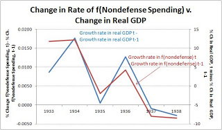
Figure 1 below shows the right hand side of equation (2) on the left axis, and the left hand side of equation (2) on the right axis. (Sorry for reversing axes, but since the right hand side of the equation (2) leads it made sense to put it on the primary axis.)
Notice that the changes in nondefense spending growth and the changes in the rate of real GDP growth correlate very strongly, despite the fact that the former is essentially determined a year and two years in advance of the latter.
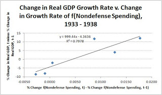
Here’s the same information with a scatterplot:
So far, it would seem that either the government’s changes to nondefense spending growth were a big determinant of real economic growth, or there’s one heck of a coincidence, particularly since I didn’t exactly “fit” the nondefense function.
But as I noted earlier in this post, after the first two graphs, I would step things up a notch. That means I’m going to show that the fit is even tighter than it looks based on the two graphs above. And I’m going to do so with a comment and a third graph.
Here’s the comment: 1933 figures do not provide information about how the New Deal programs worked. After all, the figures are midyear – so the real GDP growth would be growth from midyear 1932 to midyear 1933. But FDR didn’t become President until March of 1933.
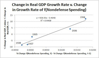
So… here’s Figure 2 redrawn, to include only data from 1934 to 1938.
While I’m a firm believer in the importance of monetary policy, for a number of reasons I don’t believe it made much of a difference in the New Deal era. As Figure 3 shows, changes in nondefense spending – hiring people to build roads, dams, and the like, explain subsequent changes in real GDP growth rates exceptionally well from 1934 to 1938. This simple model explains more than 90% of the change in real GDP growth rates over that period.
Of course, after 1938, the relationship breaks down… but by then the economy was on the mend (despite the big downturn in 1938). More importantly (I believe – haven’t checked this yet!), defense spending began to become increasingly important. People who might have been employed building roads in 1935 might have found employment refurbishing ships going to the Great Britain in 1939.
—
As always, if you want my spreadsheet, drop me a line. I’m at my first name (mike) period my last name (kimel – note only one “m”) at gmail.com.


